1.  Le modèle MPO résumé en quelques figures

• Le modèle présenté au § 6 de ’Revisiting the carbon cycle’ attribue les évolutions du CO₂ à des causes Mixtes. Les flux sortant de l’atmosphère seraient Proportionnels au taux de CO₂ atmosphérique et l’Océan serait le facteur dominant. Ce modèle est désigné ici par le sigle MPO. On reprend les simplifications de la figure 5.12 AR6 du GIEC : un modèle avec 3 compartiments (Océan, Atmosphère, Végétation/sols) et 5 flux d’échange de carbone avec l’atmosphère.

• En se restreignant à l’intervalle 1980-2025, le présent article illustre les diverses évolutions selon le modèle MPO. L’intervalle 1980-2025 permet d’utiliser, pour le taux de CO₂ atmosphérique, les 4 observatoires de base de la NOAA (BRW MLO SMO SPO) plutôt que seulement MLO. Ainsi, on peut alors utiliser exclusivement les indicateurs de température par satellites (contrairement à ‘Revisiting the carbon cycle’), ce qui peut entraîner de petites différences dans le chiffrage.

1.1 Selon le modèle MPO, les flux naturels augmentent entre 1980 et 2025

La figure ci-dessous indique les notations utilisées et présente l’évolution des 5 flux (4 flux naturels + 1 flux anthropique).

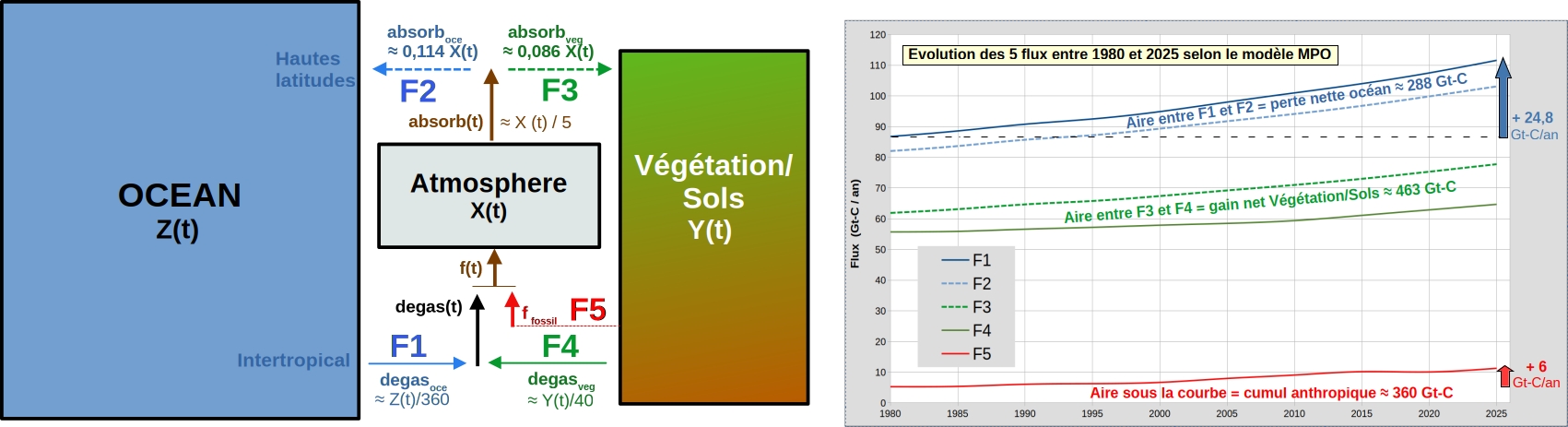
Figure 1 : à gauche, désignation simplifiée des 5 flux d’échange de carbone avec l’atmosphère. Les stocks des 3 compartiments sont X(t), Y(t), Z(t). À droite, évolution des 5 flux entre 1980 et 2025 selon le modèle MPO (1 Gt-C → 3,7 Gt-CO₂ → 0,47 ppm).

• Selon le modèle MPO, c’est le flux 1 (F1 → dégazage océanique) qui présente la plus forte augmentation en 45 ans. Entre 1980 et 2025, le flux 5 (F5 → émissions anthropiques) n’augmente que de + 6 Gt-C/an contre + 24,8 Gt-C/an pour le flux 1. Selon le modèle MPO, les croissances de X(t), F2, F3, puis de Y(t) et F4 résultent des augmentations concomitantes de F1 et F5.

• L’aire sous une courbe représente le carbone échangé par le flux avec l’atmosphère entre 1980 et 2025 : 360 Gt-C pour F5, 4652 Gt-C pour F1, 4364 Gt-C pour F2.
  Le gain net végétation/sols (463 Gt-C avec F3 > F4) et la perte nette océanique (288 Gt-C avec F1 > F2) permettent de se conformer à l’évolution mesurée de δ¹³C entre 1980 et 2025 (voir figures 5 et 6).

1.2 Une analogie avec un réservoir d’eau

L’analogie ci-dessous propose une interprétation des augmentations des flux naturels F2, F3 et F4.

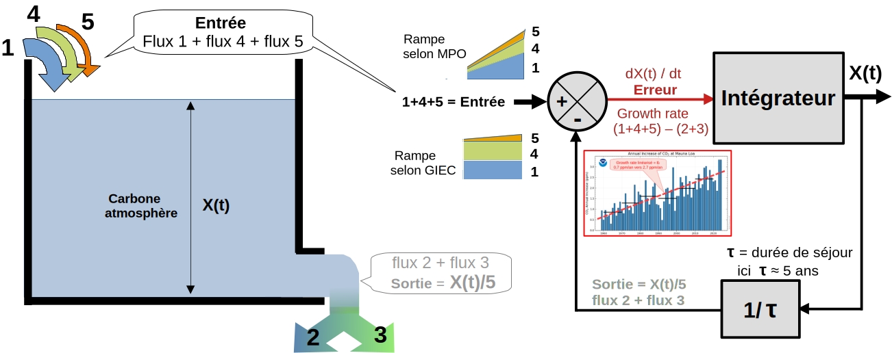
Figure 2 : Analogie avec un réservoir (à gauche) ; Modèle de l’atmosphère selon fig.14 de Revisiting the carbon cycle, avec Growth rate mesuré à Mauna Loa dans l’encadré rouge (à droite).

• La hauteur d’eau = X(t) dans le réservoir détermine la pression, laquelle commande le débit de sortie = F2 + F3.
  C’est la différence entre flux d’entrée (1+4+5) et flux de sortie (2+3) qui provoque le changement annuel de X(t), c’est-à-dire Growth rate = dX(t)/dt avec dt = 1 an. Notons que le seul flux connu à ± 5 % est le flux 5 (émissions anthropiques).
  
• En automatique linéaire, une entrée/commande qui croît quasi linéairement est appelée ‘rampe’. Selon le GIEC, la croissance en entrée (voir les 2 rampes du schéma-bloc fig. 2) est causée par le seul flux 5. Mais selon MPO, elle est causée principalement par le flux naturel F1 qui entraîne la croissance de F2 et F3 puis, à terme, la croissance de F4.

• Dans le cadre des systèmes asservis et du modèle MPO, on peut alors interpréter la croissance annuelle comme une erreur de traînage/vitesse. Entre 1980 et 2025, les entrées croissantes (la cause) ne seraient jamais rattrapées par les sorties qui augmenteraient comme X(t)/5 (la conséquence). L’analogie avec un réservoir aide à la compréhension mais reste imparfaite, car le fonctionnement réel est moins simple que le schéma-bloc de la fig. 2.

2.  Évolutions 1980-2025 pour 5 flux et 3 stocks

2.1 Illustrations des évolutions 1980-2025 selon MPO

• Les figures qui suivent illustrent l’évolution des 5 flux, de δ¹³C et des stocks X(t) Y(t) Z(t) dans les 3 compartiments.
  Les valeurs du compartiment Atmosphère (taux de CO₂ et δ¹³C) sont issues des mesures (plusieurs observatoires).
  Les valeurs pour le flux 5 (émissions anthropiques) sont issues des données de CDIAC + BP statistical review.

Toutes les autres valeurs sont estimées via la modélisation MPO et ne résultent donc pas de l’observation.

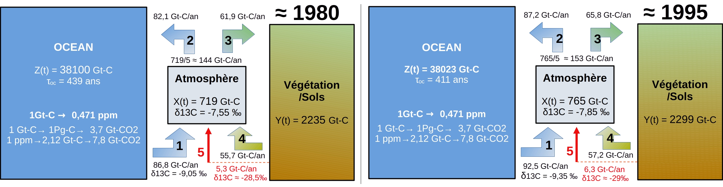
Figure 3a : Estimations selon MPO des stocks dans les 3 compartiments et des 5 flux d’échange de carbone vers 1980 et vers 1995.

• Pour la figure illustrant la situation vers 1995, on détaille ci-dessous le calcul des estimations selon le modèle MPO.
  Les flux sortant de l’atmosphère correspondent à 1/5 de X(t) = stock dans l’atmosphère : F2 + F3 = 765/5 = 153 Gt-C/an.
  Le flux F2 vers l’océan est pris comme 11,4 % du stock dans l’atmosphère : F2 = 765 * 0,114 = 87,2 Gt-C/an.
  Le flux F3 vers Végétation/Sols est pris comme 8,6 % du stock dans l’atmosphère : F3 = 765 * 0,086 = 65,8 Gt-C/an.
  On rappelle que cette procédure d’estimation est quasi compatible avec les rapports WG1 du GIEC (fig.4 de 2/3).

• Les stocks Z(t) dans l’océan et Y(t) dans Végétation/sols sont déduits des valeurs de l’année précédente : chaque année Z(t) diminue de (F1 – F2) et Y(t) augmente de (F3 – F4).

• Le flux F4 est pris comme environ 1/40 de Y(t) : F4 = 2299/40,3 = 57,2 Gt-C/an.
  Le dégazage océanique F1 dépend de la température via τ_oc → F1 = Z(t) / τ_oc = 38023 / 411 = 92,5 Gt-C/an.
  Pour le flux F1 (voir fig 8 ici), δ¹³C est inférieur de 1,5 ‰ à celui de l’atmosphère : -7,85 – 1,5 = -9,35 ‰. 

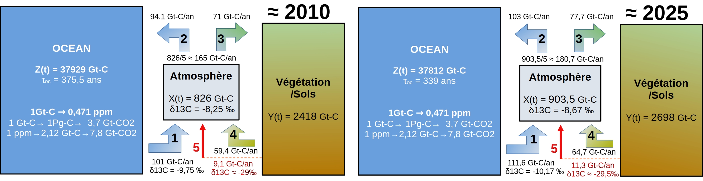
Figure 3b : Estimations selon MPO des stocks dans les 3 compartiments et des 5 flux d’échange de carbone vers 2010 et vers 2025.

• Le document Addendum.pdf détaille la méthode d’estimation des échanges naturels de carbone selon le modèle MPO.

• Selon MPO, les 45 ans d’échanges de carbone entre 3 compartiments peuvent se résumer ainsi :
  – La croissance du dégazage océanique (F1 croît de + 24,8 Gt-C/an entre 1980 et 2025) a provoqué l’augmentation de X(t) et donc aussi des flux 2 et 3. La croissance du flux 3 entraîne l’augmentation de Y(t) qui provoque celle du flux 4.
  – La croissance du flux anthropique F5 a participé plus modestement à ces augmentations (F5 croit seulement de + 6 Gt-C/an entre 1980 et 2025).

2.2 Les bilans 1980-2025 selon le modèle MPO

• On présente ci-dessous le bilan global de 45 ans d’échanges de carbone par les 5 flux entre 1980 et 2025.

Figure 4 : Cumuls des 5 flux entre 1980 et 2025 (aires sous les courbes de la fig.1) et gains ou pertes des 3 compartiments.

• Entre 1980 et 2025, l’océan dégazerait 4652 Gt-C en zone intertropicale mais absorberait 4364 Gt-C dans les hautes latitudes. En 45 ans, l’océan perdrait donc 4652 – 4364 = 288 Gt-C, soit seulement 0,76 % du carbone océanique. Selon MPO, l’océan est une source nette de carbone vis-à-vis de l’atmosphère (en désaccord avec le modèle du GIEC mais en accord avec l’évolution mesurée de δ¹³C).

• Entre 1980 et 2025, le stock de carbone atmosphérique passe de 718,7 Gt-C à 903,5 Gt-C, soit un apport ≈ 185 Gt-C. En utilisant les 5 cumuls de la fig.4, on détaille ci-dessous cet apport net de 185 Gt-C dans l’atmosphère.

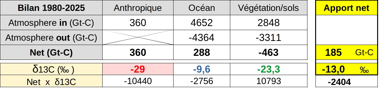
Figure 5a : Le modèle MPO → Estimation de l’apport net 1980-2025 dans l’atmosphère → 360 + 288 – 463 = 185 Gt-C. À partir des différents δ¹³C, on estime δ¹³C pour cet apport net → -10440 – 2756 + 10793 = -2404 et -2404/185 ≈ -13,0 ‰.. Koutsoyiannis 2024aobtient dans sa figure 10 des valeurs similaires pour les apports net : -12,9 ‰ > δ¹³C > -13,3 ‰.

2.3 Le modèle du GIEC semble incompatible avec les observations de δ¹³C

• Selon la thèse du GIEC, entre 1980 et 2025, les émissions anthropiques apportent 360* Gt-C à l’atmosphère dont environ la moitié serait absorbée à parts égales par Océan et Végétation/sols.
  

*Selon World Energie Outlook. ~1260 Gt-CO₂ soit ~343 Gt-C, mais le GIEC ajoute environ 5 % de LUC→343 * 1,05 ≈ 360 Gt-C.

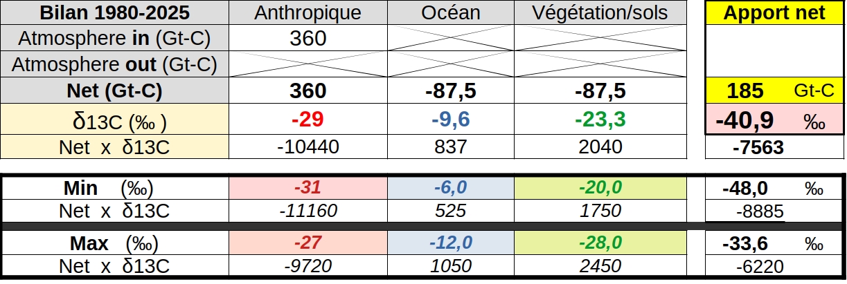
Figure 5b : Estimation, selon le modèle du GIEC, de l’apport net 1980-2025 dans l’atmosphère → 360 – 87,5 – 87,5 = 185 Gt-C. À partir des différents δ¹³C, on estime δ¹³C pour cet apport net →-10440+837+2040=-7563 et -7563/185 ≈ -40,9 ‰.. En partie basse, on montre que δ¹³C de l’apport net GIEC reste éloigné de -13 ‰ (-48 ‰ à -33,6 ‰), même pour une large plage de valeurs δ¹³C.

On vérifie ci-dessous qu’un apport net = 185 Gt-C avec δ¹³C = -13 ‰ (apport net mixte → océan + anthropique selon MPO) permet bien de retrouver la valeur observée en 2025 : δ¹³C = -8,67 ‰. En revanche, l’apport net GIEC (185 Gt-C avec δ¹³C = -40,9 ‰) ne permet pas de retrouver δ¹³C = -8,67 ‰ en 2025.

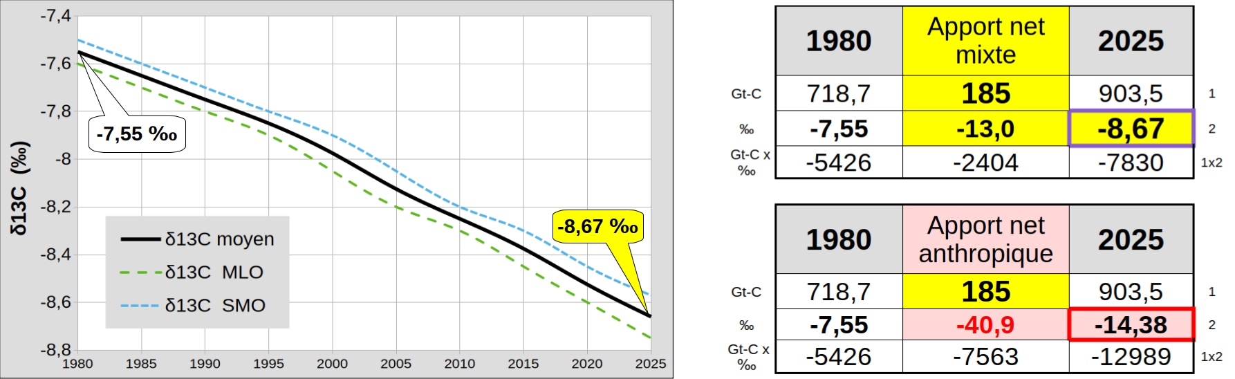
Figure 6 : à gauche →évolution (moyenne 2 hémisphères) mesurée pour δ¹³C (voir ici).
à droite →δ¹³C calculé pour l’atmosphère de 2025 selon MPO (apport net mixte) et selon GIEC (apport net anthropique)

• La thèse du GIEC est incorrecte, car un apport net de 185 Gt-C uniquement anthropique (fig.5b → δ¹³C compris entre 48 ‰ et -33,6 ‰) implique pour l’atmosphère de 2025 :  -15,8 ‰ < δ¹³C < -12,9 ‰, incompatible avec δ¹³C = -8,67 ‰.

2.4 Le modèle MPO, une ébauche compatible avec les observations

• La figure 4 montre que les compartiments Atmosphère (+185 Gt-C ou +25,6 %) et Végétation/sols (+463 Gt-C ou + 20,7 %) ont reçu des apports nets de carbone (1980-2025) provenant de l’océan et des émissions anthropiques.
  La figure ci-dessous détaille la répartition (en Gt-C, en 2025 et selon le modèle MPO) de ces 2 apports nets.

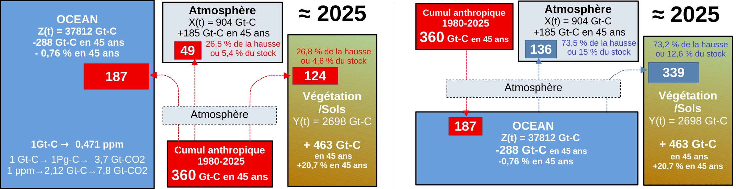
Figure 7 : Où se trouve en 2025 le carbone anthropique (360 Gt-C) apporté (1980-2025) par le flux 5 (à gauche en Gt-C) ? Où se trouve en 2025 le carbone océanique apporté en net (1980-2025) par le flux 1 (à droite en Gt-C) ?

• Contrairement au modèle du GIEC (fig.6), le modèle MPO est compatible avec les observations modernes (taux et δ¹³C) du CO₂ atmosphérique. Le modèle MPO n’utilise pas les notions et concepts imaginés par le GIEC/ONU tels : Airborne fraction, fonction de Berne, durée d’ajustement, facteur tampon de Revelle.
  Néanmoins, les très grandes incertitudes sur les échanges naturels de carbone rendent toute modélisation hasardeuse. Au mieux, on peut espérer obtenir une représentation simplifiée du cycle du carbone à l’échelle de quelques décennies.

• Parmi les pistes pour améliorer l’ébauche que constitue le modèle MPO, on peut lister :

i) Un apport de carbone depuis la lithosphère vers l’océan peut exister et ne pas être négligeable (activité volcanique sous-marine, dégazage mantellique par les fumeurs hydrothermaux des dorsales océaniques). 
ii) Les compartiments selon le GIEC doivent être revus → le compartiment atmosphère est divisible entre basse et haute atmosphère. La plupart des échanges de carbone avec Océan et Végétation/Sols ont lieu dans la basse atmosphère avec une durée de séjour ≈ 3 à 5 ans. Avec la haute atmosphère, ces échanges sont plus lents et la durée de séjour > 10 ans comme le suggèrent les mesures après 1963 sur le ¹⁴C (essais atomiques).
iii) Le flux F4, fonction de Y(t), doit dépendre aussi de la température et de l’activité biologique.
iv) Le flux F1, fonction de Z(t) et de la température SSTi, peut également dépendre de l’activité biologique en surface de l’océan intertropical.
v) Les rapports entre X(t) et F2 ou F3 (11,4 % ou 8,6%) peuvent évoluer avec le temps.

3. Réponses à quelques objections courantes

• Le modèle MPO utilise une durée de séjour de 5 ans, c’est-à-dire que, chaque année, 1/5 du carbone atmosphérique serait fixé par les compartiments Océan et Végétation/Sols. On rappelle que cette hypothèse est quasi compatible avec les 6 rapports WG1 du GIEC (fig.4 du 2/3).
  On peut néanmoins objecter que la durée de séjour n’est pas égale à 5 ans. La figure ci-dessous montre que la part anthropique (dXfossil/dt) dans la croissance annuelle (dX(t) /dt) change en effet avec la durée de séjour (4 ans à 6 ans), mais que cette variation reste très faible.

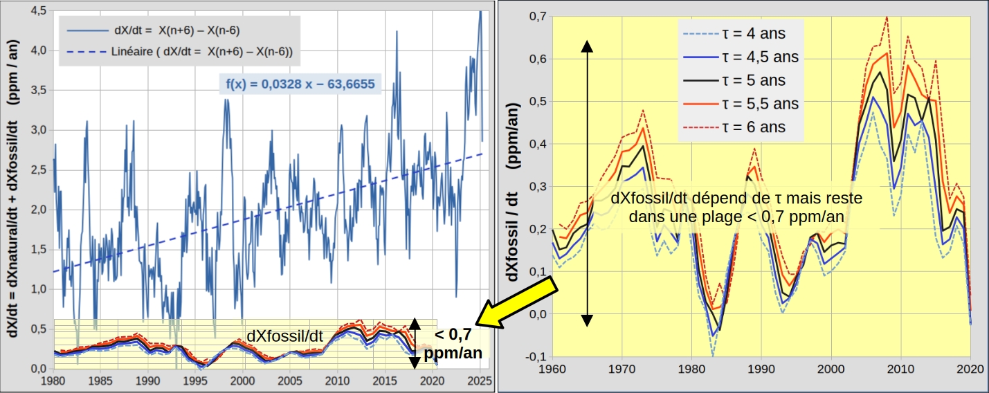
Figure 8a : à gauche : croissance du CO₂ atmosphérique = croissance naturelle + croissance anthropique →dX(t)/dt = dXnatural/dt + dXfossil/dt. à droite, la part anthropique de la croissance (dXfossil/dt) dépend de la durée de séjour mais reste dans une plage de variation ≤ 0,7 ppm/an.

• On liste ci-dessous quelques objections courantes, réfutées au §10 de ‘Revisiting the Carbon Cycle‘ ou bien réfutées dans des articles SCE. Pour les réponses à d’autres objections, le lecteur peut consulter SCE_03/2025.
  

3.1 Objections basées sur l’interprétation hâtive des observations

• a) L’objection principale au modèle MPO est la suivante : une diminution du pH moyen de l’océan suffirait pour démontrer qu’il est un puits net de carbone et non une source nette vis-à-vis de l’atmosphère.
  Ce point est contesté dans les 4 pages du § 8 de ‘Revisiting the Carbon Cycle’ : « +1°K on T or +8 μmol/kg on the DIC have about the same effect: +18 μatm on the sea water partial pressure and –0.016 on the pH » (page 157).
  Les trois remarques ci-dessous incitent également à la prudence :

i)  On peut avoir un apport de carbone depuis la lithosphère vers l’océan (activité sous-marine, fumeurs hydrothermaux des dorsales océaniques). Si cet apport* est supérieur au dégazage net (6,4 Gt-C/an→288 Gt-C en 45 ans ), alors le pH océanique diminue, même si l’océan est une source nette vis-à-vis de l’atmosphère (ici §5).

*Un faible apport (actuellement non chiffrable par défaut de mesures) compris entre 6,4 Gt-C /an et 10 Gt-C/an (flux anthropique) serait suffisant.

ii)  La précision et l’échantillonnage des mesures de pH sont-ils suffisants pour attester d’une baisse du pH moyen dans la totalité de l’océan ? voir SCE_06/2018.

iii)  Une baisse du pH peut aussi résulter d’une modification de l’équilibre physico-chimique du carbone dans l’océan via la hausse de la température SSTi (exemple ci-dessous avec le simulateur Alkalinity-Temperature-DIC).

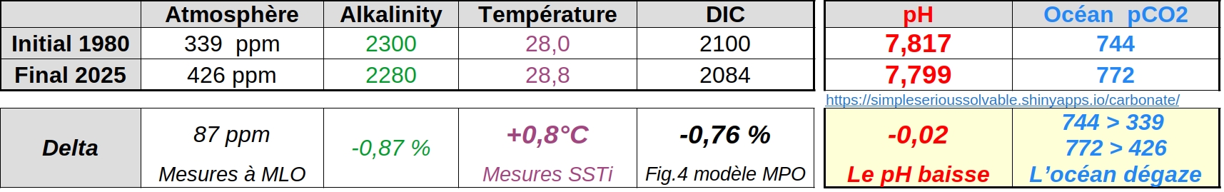
Figure 8b : Un exemple de conditions pour lesquelles le pH baisse et l’océan dégaze → DIC baisse de 0,76 % : voir simulateur.
 

• b) Le CO₂ atmosphérique s’appauvrit en ¹³C.
  Les observations montrent en effet un appauvrissement, mais il est trop lent pour être causé uniquement par les émissions anthropiques : voir fig.6 ; également §7 de ‘Revisiting the Carbon Cycle‘ ou bien §4 de SCE_03/25 ainsi que pages 22-24 dans The Cause Of Earth’s Climate Change Is The Sun.
  
• c) Le CO₂ atmosphérique s’appauvrit en ¹⁴C.
  Les observations montrent bien un appauvrissement, mais celui-ci ne peut pas être causé uniquement par les émissions anthropiques : voir §11 de ‘Revisiting the Carbon Cycle‘ ainsi que §5 de SCE_06/19.

3.2 Objections fondées sur les concepts initiés par le GIEC/ONU

a) ‘Airborne Fraction’: selon le GIEC/ONU, il resterait environ 44 % des émissions anthropiques dans l’atmosphère sans qu’il en soit de même pour les émissions naturelles.
En réalité, il reste chaque année dans l’atmosphère l’équivalent d’environ 1 à 4 % des émissions, naturelles et  anthropiques. Voir §10.4 dans ‘Revisiting the Carbon Cycle‘ ainsi que les figures 2a 2b dans SCE_01/24.

b) ‘Bern function’ : théorie d’une réponse logarithmique lente du CO₂ dans l’atmosphère.
Ces fonctions de Berne sont contraires aux observations : voir § 10.5 de ‘Revisiting the Carbon Cycle‘ ainsi que SCE_07/19.

c) ‘Adjustment time’ (50 – 200 ans) ou stock persistant de CO₂ anthropique.
Le concept ‘adjustment time’ est contestable, surtout en l’absence d’équilibre préalable. Voir § 10.6 et 10.7 de ‘Revisiting the Carbon Cycle‘ ou § 1.4.2 page 35 de The  Rational Climate e-Book ou § 3 de Koutsoyiannis 2024b.

d) ‘Revelle factor’ ou ‘Buffer factor’, “bottleneck” entre atmosphère et océan.
Ces concepts sont inapplicables dans le monde réel (température ni constante ni homogène) : voir §8 et §10.8 dans ‘Revisiting the Carbon Cycle‘ ainsi que The  Rational Climate e-Book (pages 289-290). 

• Ces quatre concepts introduits par le GIEC/ONU semblent, en définitive, être des constructions ad hoc.
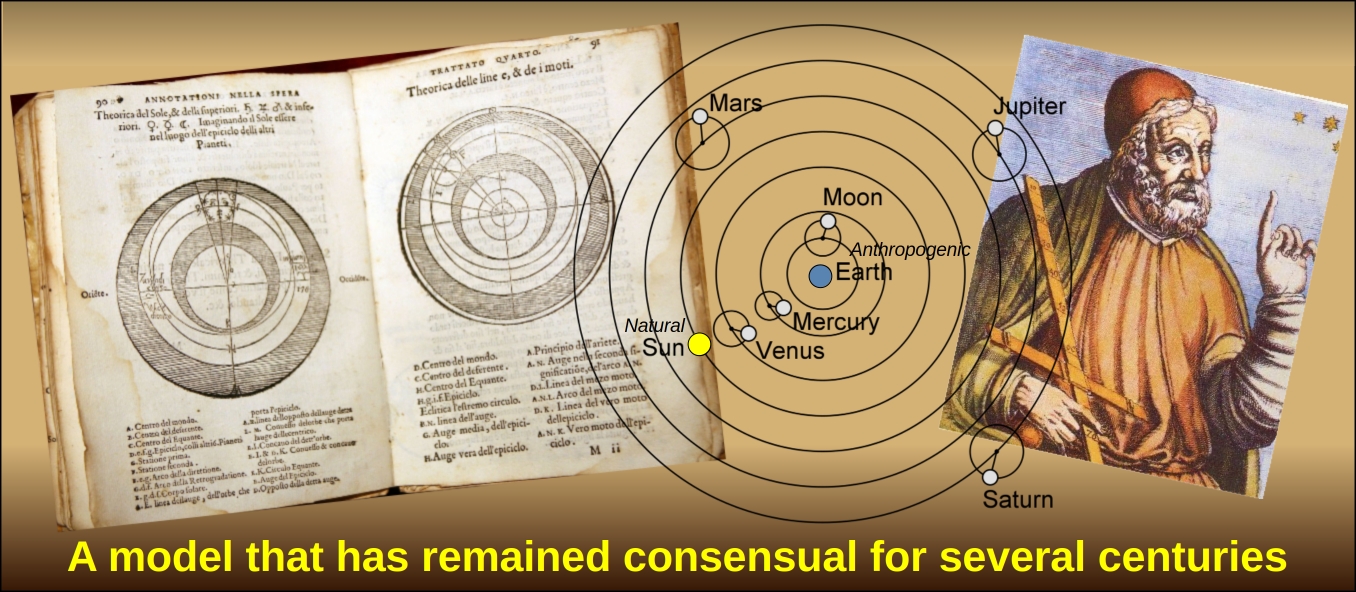
  Ils jouent un rôle comparable (dans le système de Ptolémée) à celui des épicycles et des déférents, ces chimères qui permettaient de maintenir le dogme des mouvements exclusivement circulaires autour d’une Terre centrale.

3.3 Le passé éclaire-t-il le présent ?

• Au Quaternaire, se succèdent des épisodes glaciaires (≈ 90 ka, végétation prostrée) et des épisodes interglaciaires (≈ 15 ka, végétation plus abondante). Schématiquement, lors des diverses transitions glaciaire → interglaciaire, on a nécessairement un transfert de carbone (CO₂) depuis le compartiment Océan vers le compartiment Végétation/Sol tandis que la température et les précipitations augmentent.
  Par exemple, lors de la dernière transition entre -15 ka BP et -10 ka BP on observe simultanément une augmentation du niveau marin ≈ +120 m et de la température moyenne globale ≈ + 5 °C (mais ≈ + 9°C au Spitzberg et N Canada).
  Selon MPO, entre 1980 et 2025, le même phénomène global (transfert de carbone océanique (CO₂) vers Végétation/sols) se produit, mais à une échelle plus réduite (≈ + 0,8 °C en un demi-siècle pour la température moyenne globale). 

• Si l’augmentation du CO₂ atmosphérique lors des dernières décennies est bien majoritairement naturelle, alors elle a dû se produire à plusieurs reprises lors de l’Holocène (ici fig.4.4). Cette hypothèse semble apparemment contredite par le proxy microbulle d’air dans les archives glaciaires (mais ce proxy est mis en cause ici § 1.5.5.2 ou bien là). En revanche, le proxy stomates (ici ou là) ou les mesures directes avant 1957 (ici) montrent que des taux de CO₂ > 350 ppm lors de l’Holocène ne peuvent pas être exclus. Si ces variations du CO₂ atmosphérique n’entraînent pas un réchauffement particulièrement inquiétant au cours de l’Holocène (ici § 1.5.1.2), il est alors nécessaire de douter des projections extrêmes avancées par le GIEC/ONU.
  
• Ces projections s’appuient sur les notions de ‘radiative forcing’ et ‘greenhouse effect’. Elles se fondent ainsi sur des modèles contestables promus par une science encore jeune, largement soutenue par un consensus politique. Un soutien qui semble égarer cette discipline récente vers une soumission aux modèles plutôt qu’aux observations.
  Des publications récentes montrent aussi que l’on peut douter de l’hypothèse centrale du GIEC, c’est-à-dire un réchauffement climatique causé par les émissions anthropiques de CO₂ .

4.  Conclusions

• Le modèle MPO est guidé par les observations modernes : évolutions de δ¹³C (fig.5 et 6) et corrélations (fig.6e du 1/3). Selon ce modèle, tous les flux d’échange de carbone avec l’atmosphère croissent entre 1980 et 2025. Cette croissance résulte surtout de la hausse de température de l’océan intertropical et marginalement du flux anthropique.

• Dans le § 2.1 du présent article, le modèle MPO se montre compatible avec les mesures modernes(taux et δ¹³C) du CO₂ atmosphérique. On y propose une estimation des flux naturels (Addendum.pdf) et des stocks entre 1980 et 2025.

• Dans le § 2.2, on présente divers bilans (1980-2025) qui démontrent la cohérence interne du modèle MPO. Cependant, la cohérence d’un modèle n’est pas une preuve de sa validité. Par ailleurs, les incertitudes sur les flux naturels incitent à la prudence : au mieux, le modèle MPO est une simplification du monde réel, valable sur quelques décennies.

• Ce modèle est une première ébauche reprenant les 3 compartiments et 5 flux du GIEC, mais c’est une ébauche guidée par des mesures modernes fiables plutôt que par des proxies incertains. L’hypothèse centrale (20 % du carbone atmosphérique est fixé chaque année : 11,4 % par l’Océan et 8,6% par Végétation/Sols) est quasi compatible avec les 6 rapports WG1 du GIEC (fig. 4 du 2/3).

• Le § 3 répond aux principales critiques adressées au modèle MPO. Elles résultent souvent d’interprétations hâtives des observations ou bien d’invocations de concepts ad hoc initiés par le GIEC.

• Le § 10 de ‘Revisiting the carbon cycle‘ conteste ces concepts du GIEC/ONU (ils confortent l’anthropocentrisme inscrit dans le rôle du GIEC). En effet, le GIEC/ONU présuppose une influence centrale de l’homme, en adoptant une vision fixiste des flux naturels. Selon ce présupposé, le seul changement notable proviendrait du flux anthropique tandis que les flux naturels resteraient quasi fixes et équilibrés.

• Jadis, les déférents et épicycles justifiaient un dogme millénaire : celui de mouvements circulaires autour d’une Terre centrale. De nos jours, les concepts ‘radiative forcing’ et ’airborne fraction’ valideraient la science ‘settled’ du GIEC/ONU. Mais ces nouveaux épicycles risquent fort de tourner court → d’ici quelques COP, un historien malicieux pourrait bien proposer pour le GIEC un nom plus approprié : Institut Ptolémée pour la Condamnation du Carbone.

La partie 1 de l’article expose les raisons qui ont guidé vers le modèle (étude des corrélations et δ¹³C).
La partie 2 de l’article présente le modèle utilisé dans les figures 14 et 15 du § 6 de ‘Revisiting the carbon cycle’.

Références

Revisiting the carbon cycle (C. Veyres, JC Maurin, P. Poyet, 2025)
(Quay et al., 2003, p.4-12) Fig. 8   https://doi.org/10.1029/2001GB001817
(Haverd et al,2019) Fig. 2  https://onlinelibrary.wiley.com/doi/pdfdirect/10.1111/gcb.14950
(Kouwenberg et al,2005) Fig.3  Atmospheric CO₂ fluctuations during the last millennium

What Causes Increasing Greenhouse Gases? (Salby, Harde, 2022)
A Nobel Prize for Climate Models Errors (R. Clark, 2024)
Koutsoyiannis 2024a
Koutsoyiannis 2024b 
Le château de carte du réchauffement anthropique (C. Veyres)
The Rational Climate e-Book  (P. Poyet, 2022)
Les Alarmistes malades de la Presse  (JC Maurin, 2026)

Addendum en français : Addendum.pdf

‘Revisiting the carbon cycle’ (3/3)

3/3  Additions, illustrations, responses to objections

Within the span of a few decades, a simple hypothesis—that the rise in atmospheric CO2 is due solely to human emissions—has become widely accepted thanks to the political influence of the UN/IPCC. However, in 2025, a study titled “Revisiting the Carbon Cycle” called into question the carbon cycle model endorsed by the IPCC. In fact, in paragraph 6, the study proposes a model that competes with the IPCC’s. This new model argues that the rise in atmospheric CO₂ is primarily determined by the surface temperature of the intertropical ocean (anthropogenic emissions are only a secondary factor). The model is presented here in three parts: Part 1 explains the reasons behind it, Part 2 provides a brief description. This Part 3 illustrates the changes in carbon flows according to this model and then addresses the main criticisms leveled against it. PDF version here.

1. The MPO model summarized in a few figures

• The model presented in Section 6 of “Revisiting the carbon cycle” attributes changes in CO₂ to Mixed causes. Flows out of the atmosphere are assumed to be Proportional to the atmospheric CO₂ concentration, with the Ocean being the dominant factor. This model is referred to here by the acronym MPO. We adopt the simplifications from IPCC AR6 Figure 5.12: a model with 3 compartments (Ocean, Atmosphere, Vegetation/Soils) and 5 carbon exchange flows with the atmosphere.

• Limiting the analysis to the 1980–2025 period, this article illustrates the various trends according to the MPO model. The 1980–2025 period allows us to use the four basic NOAA observatories (BRW, MLO, SMO, SPO) for atmospheric CO₂ concentrations rather than just MLO. Thus, we can rely exclusively on satellite-based temperature data (unlike in “Revisiting the carbon cycle”), which may result in slight differences in the estimates.

1.1 According to the MPO model, natural fluxes increase between 1980 and 2025

The figure below explains the notation used and shows the trends for the five fluxes (four natural fluxes + one anthropogenic flux).

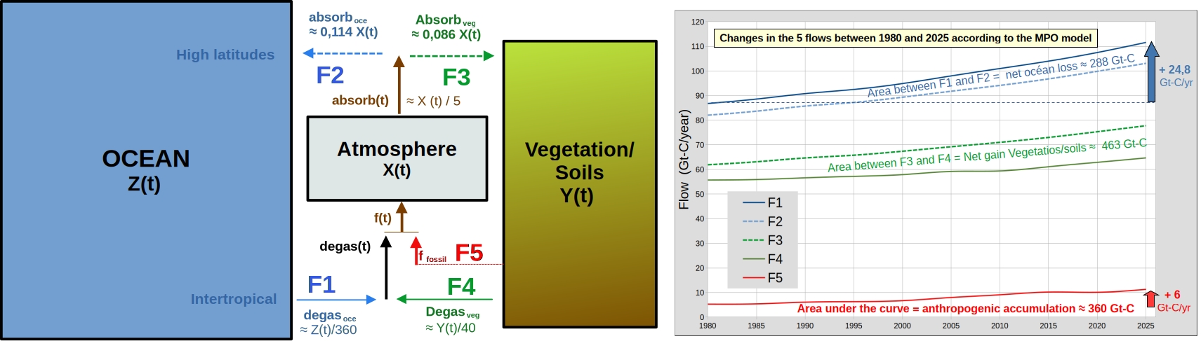
Figure 1: On the left, a simplified diagram of the five carbon exchange fluxes with the atmosphere. The stocks of the three compartments are X(t), Y(t), Z(t). On the right, changes in the five fluxes between 1980 and 2025 according to the MPO model (1 Gt-C → 3.7 Gt-CO2 → 0.47 ppm).

• According to the MPO model, flux 1 (F1 → ocean degassing) shows the greatest increase over 45 years. Between 1980 and 2025, flux 5 (F5 → anthropogenic emissions) increases by only +6 Gt-C/year, compared to +24.8 Gt-C/year for flux 1. According to the MPO model, the increases in X(t), F2, F3, and then Y(t) and F4 result from the concomitant increases in F1 and F5.

• The area under a curve represents the carbon exchanged by the flux with the atmosphere between 1980 and 2025: 360 Gt-C for F5, 4,652 Gt-C for F1, 4,364 Gt-C for F2. The net gain from vegetation/soils (463 Gt-C with F3 > F4) and the net loss from the ocean (288 Gt-C with F1 > F2) are consistent with the measured trend in δ¹³C between 1980 and 2025 (see Figures 5 and 6).

1.2 An analogy with a water tank

The analogy below offers an interpretation of the increases in the natural flows F2, F3, and F4.

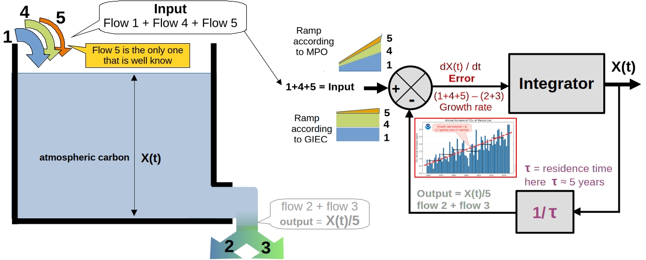
Figure 2: Analogy with a reservoir (left); Atmospheric model based on Fig. 14 from ‘Revisiting the carbon cycle‘, with the growth rate measured at Mauna Loa shown in the red box (right).

• The water level = X(t) in the reservoir determines the pressure, which controls the outflow = F2 + F3.
It is the difference between the inflow (1+4+5) and the outflow (2+3) that causes the annual change in X(t), i.e., growth rate = dX(t)/dt with dt = 1 year. Note that the only flux known to within ±5% is flux 5 (anthropogenic emissions).

• In linear control systems, an input/command that increases quasi-linearly is called a ‘ramp’. According to the IPCC, the growth in the input (see the two ramps in the block diagram in Fig. 2) is caused solely by flow 5. But according to the MPO model, it is caused primarily by the natural flux F1, which drives the growth of F2 and F3 and, ultimately, the growth of F4.

• In the context of controlled systems and the MPO model, the annual growth can then be interpreted as a tracking error. Between 1980 and 2025, the increasing inputs (the cause) would never be offset by the outputs, which would increase as X(t)/5 (the consequence). The analogy with a reservoir aids understanding but remains imperfect, as the actual operation is less simple than the block diagram in Fig. 2.

2. Trends from 1980 to 2025 for 5 fluxes and 3 stocks

2.1 Illustrations of trends from 1980 to 2025 according to MPO

• The following figures illustrate the trends in the 5 fluxes, δ¹³C, and the stocks X(t), Y(t), and Z(t) across the 3 compartments.
The values for the Atmosphere compartment (CO₂ concentration and δ¹³C) are derived from measurements (from multiple observatories). The values for flux 5 (anthropogenic emissions) are derived from CDIAC data and the BP Statistical Review.
All other values are estimated using MPO modeling and are therefore not based on observations.

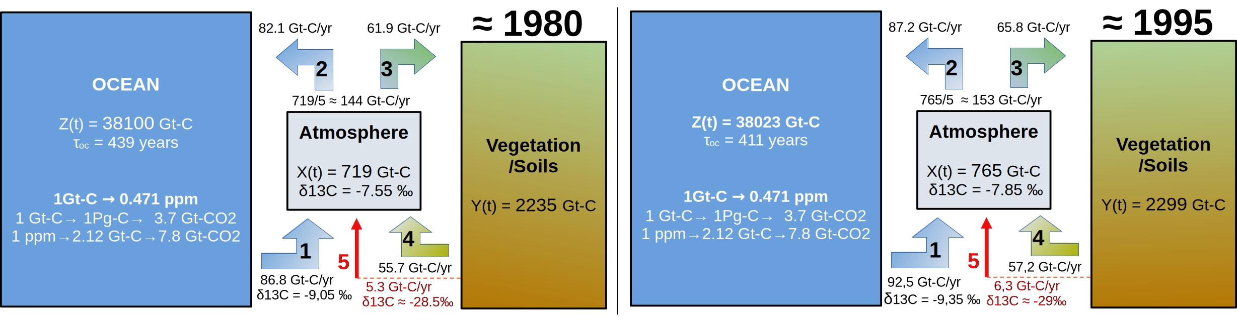
Figure 3a: MPO estimates of carbon stocks in the three compartments and of the five carbon exchange fluxes around 1980 and around 1995.

• For the figure illustrating the situation around 1995, the calculation of the estimates based on the MPO model is detailed below. Flows leaving the atmosphere correspond to 1/5 of X(t) = atmospheric stock: F2 + F3 = 765/5 = 153 Gt-C/year.
The flux F2 to the ocean is taken as 11.4% of the atmospheric stock: F2 = 765 * 0.114 = 87.2 Gt-C/year.
The flux F3 to Vegetation/Soils is taken as 8.6% of the atmospheric stock: F3 = 765 * 0.086 = 65.8 Gt-C/year.
It should be noted that this estimation procedure is largely consistent with the IPCC WG1 reports (Fig. 4 of 2/3).

• The stocks Z(t) in the ocean and Y(t) in Vegetation/Soils are derived from the previous year’s values: each year Z(t) decreases by (F1 – F2) and Y(t) increases by (F3 – F4).

• The flux F4 is taken as approximately 1/40 of Y(t): F4 = 2299/40.3 = 57.2 Gt-C/year.
Oceanic degassing F1 depends on temperature via τ_oc → F1 = Z(t) / τ_oc = 38023 / 411 = 92.5 Gt-C/year. For flux F1 (see Fig. 8 here), δ¹³C is 1.5 ‰ lower than that of the atmosphere: -7.85 – 1.5 = -9.35 ‰.

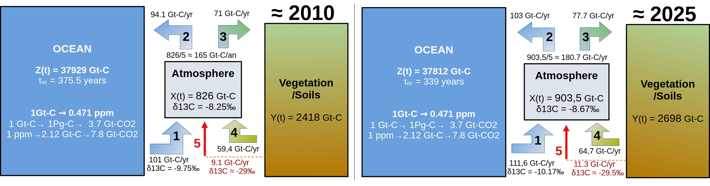
Figure 3b: MPO estimates of stocks in the three compartments and the five carbon exchange fluxes around 2010 and around 2025.

• The document Addendum.pdf details the method for estimating natural carbon exchanges using the MPO model.

• According to MPO, the 45 years of carbon exchange between the three compartments can be summarized as follows:
– The increase in ocean degassing (F1 increases by +24.8 Gt-C/year between 1980 and 2025) caused an increase in X(t) and thus also in fluxes 2 and 3. The increase in flux 3 leads to an increase in Y(t), which in turn causes an increase in flux 4.
– The increase in anthropogenic flux F5 contributed more modestly to these increases (F5 increases by only +6 Gt-C/year between 1980 and 2025).
 

2.2 Carbon balances for 1980–2025 based on the MPO model

• The table below shows the overall carbon balance for 45 years across the five carbon fluxes between 1980 and 2025.

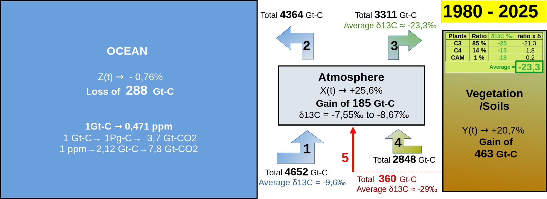
Figure 4: Cumulative totals of the five fluxes between 1980 and 2025 (areas under the curves in Fig. 1) and gains or losses in the three compartments.
 

• Between 1980 and 2025, the ocean would release 4,652 Gt-C in the intertropical zone but absorb 4,364 Gt-C in high latitudes. Over 45 years, the ocean would thus lose 4,652 – 4,364 = 288 Gt-C, or only 0.76% of oceanic carbon. According to MPO, the ocean is a net source of carbon relative to the atmosphere (contrary to the IPCC model but consistent with the measured trend in δ¹³C).
 

• Between 1980 and 2025, the atmospheric carbon stock increases from 718.7 Gt-C to 903.5 Gt-C, representing a net increase of ≈ 185 Gt-C. Using the five cumulative values from Fig. 4, we detail below this net increase of 185 Gt-C in the atmosphere.

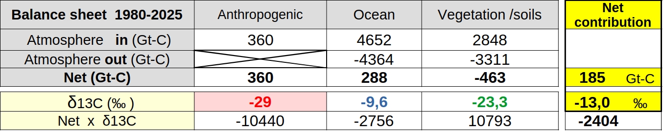
Figure 5a: The MPO model → Estimated net input to the atmosphere, 1980–2025 → 360 + 288 – 463 = 185 Gt-C. Based on the various δ¹³C values, δ¹³C is estimated for this net input → -10,440 – 2,756 + 10,793 = -2,404 and -2,404/185 ≈-13.0‰. Koutsoyiannis 2024a, reports in Fig. 10 similar values for net contributions: -12.9‰ > δ¹³C > -13.3‰.

2.3 The IPCC model appears to be inconsistent with δ¹³C observations

• According to the IPCC’s assessment, between 1980 and 2025, anthropogenic emissions will release 360* Gt-C into the atmosphere, about half of which is expected to be absorbed equally by the ocean and vegetation/soils.

* According to the World Energie Outlook, ~1,260 Gt-CO2, or ~343 Gt-C, but the IPCC adds approximately 5% for land-use change (LUC) → 343 * 1.05 ≈ 360 Gt-C.

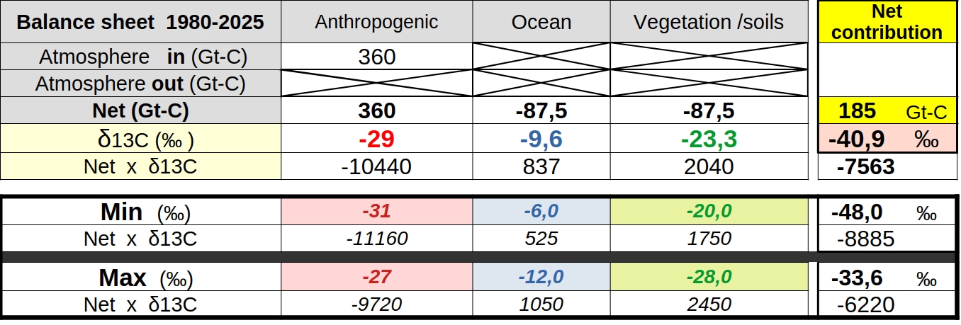
Figure 5b: Estimate, based on the IPCC model, of the net input to the atmosphere from 1980 to 2025 → 360 – 87.5 – 87.5 = 185 Gt-C. Based on the various δ¹³C values, we estimate δ¹³C for this net input → -10,440 + 837 + 2,040 = -7,563 and -7,563/185 ≈ -40.9‰. In the lower section, we show that the IPCC’s δ¹³C for the net input remains far from -13‰ (-48‰ to -33.6‰), even for a wide range of δ¹³C values.

• We verify below that a net input of 185 Gt-C with δ¹³C = -13‰ (mixed net input → ocean + anthropogenic according to MPO) does indeed reproduce the value observed in 2025: δ¹³C = -8.67‰. In contrast, the IPCC net input (185 Gt-C with δ¹³C = -40.9‰) does not yield δ¹³C = -8,67‰  in 2025.

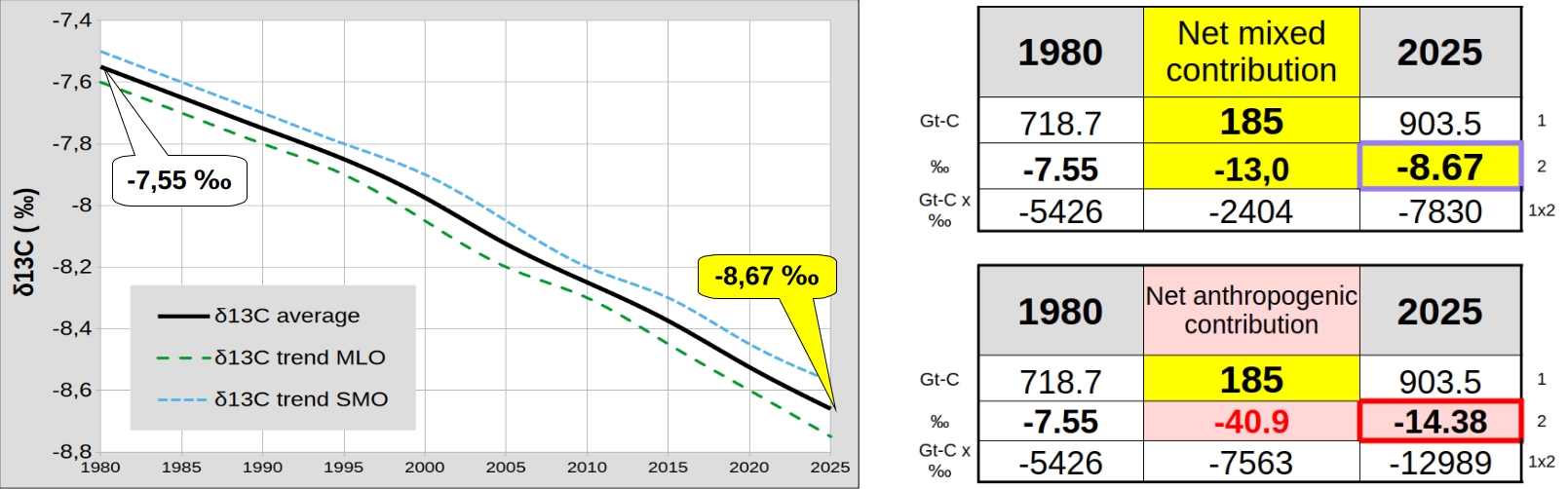
Figure 6: Left → trend (average of both hemispheres) measured for δ13C (see here).
Right → δ13C calculated for the atmosphere in 2025 according to MPO (mixed net flux) and according to the IPCC (anthropogenic net flux).

• The IPCC’s thesis is incorrect, because a net input of 185 Gt-C that is solely anthropogenic (Fig. 5b → δ¹³C between 48‰ and -33.6‰) implies for the atmosphere in 2025: -15.8 ‰ < δ¹³C < -12.9 ‰, which is incompatible with δ¹³C = -8,67‰.

2.4 The MPO model: a preliminary version consistent with observations

• Figure 4 shows that the Atmosphere (+185 Gt-C or +25.6%) and Vegetation/Soils (+463 Gt-C or +20.7%) compartments received net carbon inputs (1980–2025) from the ocean and anthropogenic emissions.
The figure below details the distribution (in Gt-C, in 2025, and according to the MPO model) of these two net inputs.

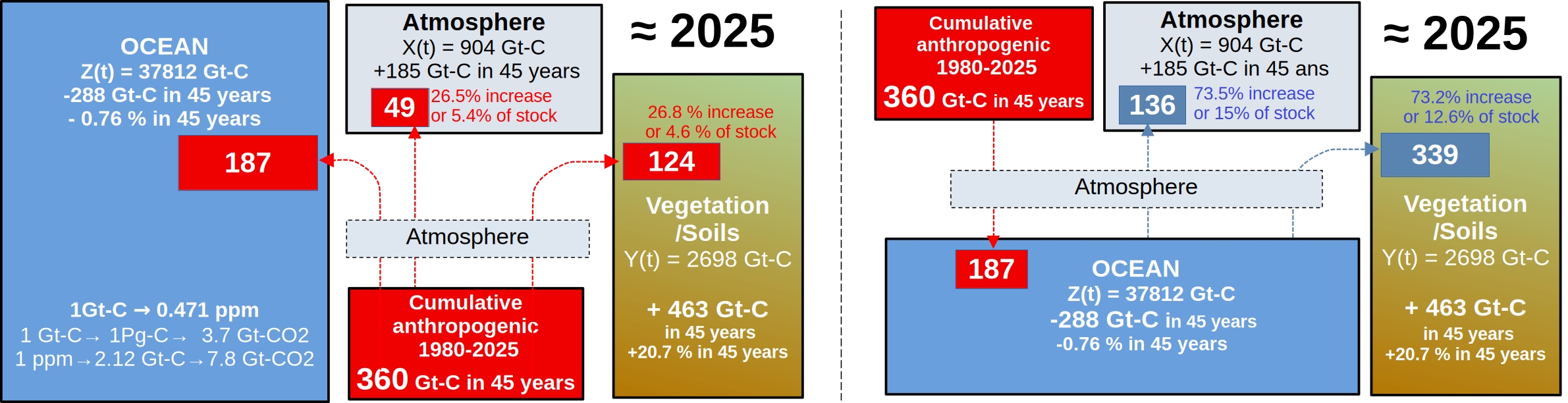
Figure 7: Where is the anthropogenic carbon (360 Gt-C) added (1980–2025) by flow 5 (on the left in Gt-C) located in 2025? Where will the net oceanic carbon (1980–2025) contributed by flux 1 (right, in Gt-C) be in 2025?

• Unlike the IPCC model (Fig. 6), the MPO model is consistent with modern observations (concentrations and δ¹³C) of atmospheric CO₂. The MPO model does not use the notions and concepts devised by the IPCC/UN, such as: airborne fraction, Bern function, adjustment time, and Revelle buffer factor.
Nevertheless, the very high uncertainties surrounding natural carbon exchanges make any modeling inherently risky. At best, we can hope to obtain a simplified representation of the carbon cycle on a timescale of a few decades.

• Among the avenues for improving the MPO model, which is still in its early stages, the following can be listed:

i) Carbon input from the lithosphere into the ocean may exist and may not be negligible (submarine volcanic activity, mantle degassing via hydrothermal vents on ocean ridges).
ii) The IPCC’s carbon pools need to be revised → the atmosphere pool can be divided into the lower and upper atmosphere. Most carbon exchanges with the ocean and vegetation/soils occur in the lower atmosphere, with a residence time of approximately 3 to 5 years. With the upper atmosphere, these exchanges are slower and the residence time is > 10 years, as suggested by post-1963 measurements of ¹⁴C (nuclear tests).
iii) Flux F4, a function of Y(t), must also depend on temperature and biological activity.
iv) The flux F1, a function of Z(t) and the SSTi temperature, may also depend on biological activity at the surface of the intertropical ocean.
v) The ratios between X(t) and F2 or F3 (11.4% or 8.6%) may change over time.

3. Responses to Some Common Objections

• The MPO model uses a residence time of 5 years, meaning that each year, 1/5 of atmospheric carbon is sequestered by the Ocean and Vegetation/Soil compartments. It should be noted that this assumption is largely consistent with the six WG1 reports of the IPCC (Fig. 4, 2/3) .
One might nevertheless object that the residence time is not exactly 5 years. The figure below shows that the anthropogenic component (dXfossil/dt) in annual growth (dX(t)/dt) does indeed vary with residence time (4 to 6 years), but that this variation remains very small.

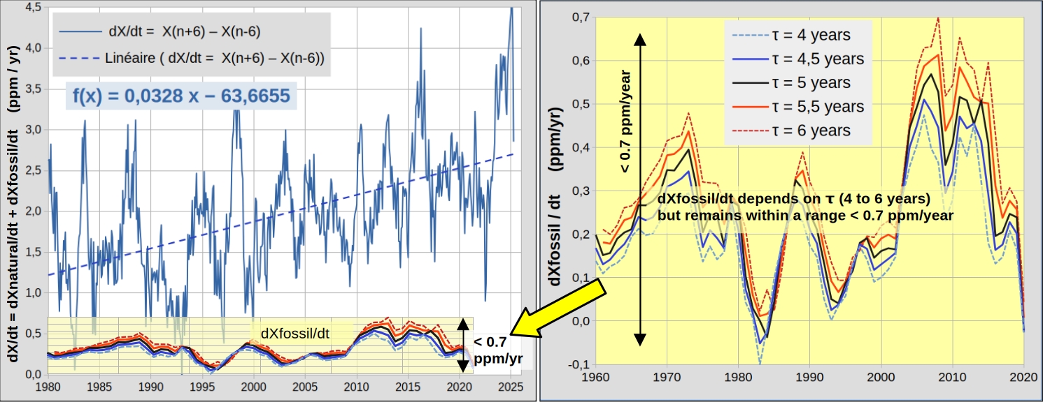
Figure 8a: Left: Atmospheric CO₂ growth = natural growth + anthropogenic growth → dX(t)/dt = dXnatural/dt + dXfossil/dt. Right: The anthropogenic component of the growth (dXfossil/dt) depends on the residence time but remains within a range of ≤ 0.7 ppm/year.

• Listed below are some common objections, refuted in §10 of ‘Revisiting the Carbon Cycle‘ or refuted in SCE articles. For responses to other objections, the reader may consult SCE_03/2025.

3.1 Objections Based on a Hasty Interpretation of Observations

• a) The main objection to the MPO model is as follows: a decrease in the average ocean pH would be sufficient to demonstrate that the ocean is a net carbon sink rather than a net source relative to the atmosphere.
This point is contested in the 4 pages of Section 8 of ‘Revisiting the Carbon Cycle’: “+1°K in T or +8 μmol/kg in DIC have about the same effect: +18 μatm in seawater partial pressure and –0.016 in pH” (page 157).
The three remarks below also call for caution:

i) There may be a carbon input from the lithosphere into the ocean (submarine activity, hydrothermal vents on ocean ridges). If this input* exceeds net degassing (6.4 Gt-C/year → 288 Gt-C in 45 years), then oceanic pH decreases, even if the ocean is a net source relative to the atmosphere (here §5).

*A small input (currently unquantifiable due to a lack of measurements) ranging from 6.4 Gt-C/year to 10 Gt-C/year (anthropogenic flux) would be sufficient.

ii) Are the accuracy and sampling of pH measurements sufficient to confirm a decrease in average pH throughout the entire ocean? See SCE_06/2018.

iii) A decrease in pH can also result from a change in the physicochemical carbon balance in the ocean via an increase in SSTi (example below using the Alkalinity-Temperature-DIC simulator).

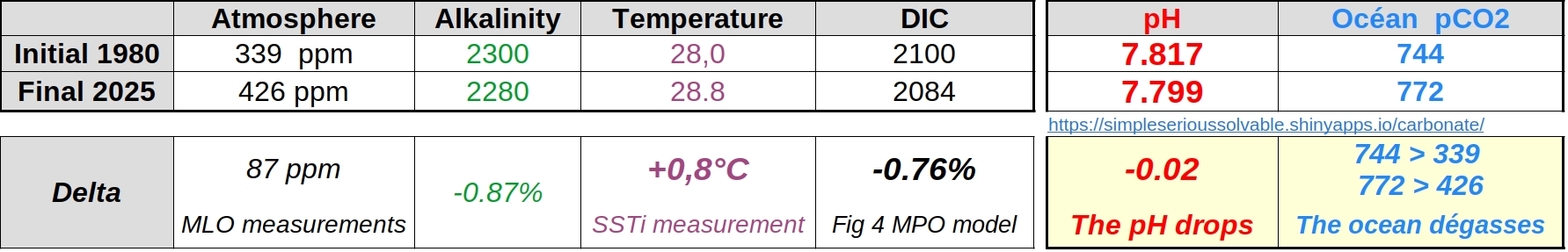
Figure 8b: An example of conditions under which the pH decreases and the ocean degasses → DIC decreases by 0.76%: see simulator.

• b) Atmospheric CO₂ becomes depleted in ¹³C.
Observations do indeed show a depletion, but it is too slow to be caused solely by anthropogenic emissions: see Fig. 6; also §7 of ‘Revisiting the Carbon Cycle’ or §4 of SCE_03/25 as well as pages 22–24 in The Cause Of Earth’s Climate Change Is The Sun.

• c) Atmospheric CO₂ is becoming depleted in ¹⁴C.
Observations do indeed show a depletion, but this cannot be caused solely by anthropogenic emissions: see §11 of ‘Revisiting the Carbon Cycle’ as well as § 5 of SCE_06/19.

3.2 Objections Based on Concepts Introduced by the IPCC/UN

a) ‘Airborne Fraction’: According to the IPCC/UN, approximately 44% of anthropogenic emissions remain in the atmosphere, whereas this is not the case for natural emissions.
In reality, the equivalent of approximately 1 to 4% of emissions—both natural and anthropogenic—remains in the atmosphere each year. See §10.4 in ‘Revisiting the Carbon Cycle’ as well as Figures 2a and 2b in SCE_01/24.

b) ‘ Bern function: theory of a slow logarithmic response of CO₂ in the atmosphere.
These Bern functions contradict observations: see § 10.5 of ‘Revisiting the Carbon Cycle’ as well as SCE_07/19.

c) ‘Adjustment time’ (50–200 years) or persistent stock of anthropogenic CO₂.
The concept of ‘adjustment time’ is questionable, especially in the absence of prior equilibrium. See Sections 10.6 and 10.7 of ‘Revisiting the Carbon Cycle’ or Section 1.4.2 on page 35 of The  Rational Climate e-Book or Section 3 of  Koutsoyiannis 2024b.

d) ‘Revelle factor’ or ‘Buffer factor’, a “bottleneck” between the atmosphere and the ocean.
These concepts are inapplicable in the real world (where temperature is neither constant nor homogeneous): see §8 and §10.8 in Revisiting the Carbon Cycle‘ as well as The  Rational Climate e-Book (pages 289–290).

• These four concepts introduced by the IPCC/UN ultimately appear to be ad hoc constructs.
They play a role comparable (in Ptolemy’s system) to that of epicycles and deferents, those fanciful constructs that allowed for the maintenance of the dogma of exclusively circular motions around a central Earth.

3.3 Does the past shed light on the present?

During the Quaternary, glacial periods (≈ 90 ka, stunted vegetation) alternated with interglacial periods (≈ 15 ka, more abundant vegetation). Broadly speaking, during the various glacial-to-interglacial transitions, there is necessarily a transfer of carbon dioxide from the ocean to the vegetation/soil compartment as temperature and precipitation increase.
For example, during the last transition between -15 ka BP and -10 ka BP, we observe a simultaneous rise in sea level ≈ +120 m and global average temperature ≈ +5°C (but ≈ +9°C in Spitsbergen and northern Canada).
According to MPO, between 1980 and 2025, the same global phenomenon (transfer of carbon dioxide from the ocean to vegetation/soils) is occurring, but on a smaller scale (≈ +0.8 °C over half a century for the global average temperature).

• If the increase in atmospheric CO₂ over the past few decades is indeed largely natural, then it must have occurred repeatedly during the Holocene (see Fig. 4.4). This hypothesis appears to be contradicted by the air microbubble proxy in ice core records (but this proxy is called into question here § 1.5.5.2 or there). On the other hand, the stomatal proxy (here or there) or direct measurements prior to 1957 (here) show that CO₂ levels > 350 ppm during the Holocene cannot be ruled out.
If these variations in atmospheric CO₂ during the Holocene do not lead to particularly alarming warming (here § 1.5.1.2), then it is necessary to question the extreme projections put forward by the IPCC/UN.

• These projections are based on the concepts of “radiative forcing” and the “greenhouse effect”. They thus rely on questionable models promoted by a still-young science, largely supported by a political consensus. This support appears to be leading this recent discipline toward submission to models rather than to empirical observations.
Recent studies also suggest that the IPCC’s central hypothesis—namely, that global warming is caused by anthropogenic CO₂ emissions—is open to question.

4 Conclusions

• The MPO model is guided by modern observations: trends in δ¹³C (Figs. 5 and 6) and correlations (Fig. 6e of the 1/3). According to this model, all carbon exchange fluxes with the atmosphere increase between 1980 and 2025. This increase results primarily from the rise in intertropical ocean temperatures and, to a lesser extent, from anthropogenic fluxes.

• In Section 2.1 of this article, the MPO model is shown to be consistent with modern measurements (concentrations and δ¹³C) of atmospheric CO₂. It provides an estimate of natural fluxes (Addendum.pdf) and stocks between 1980 and 2025.

• In Section 2.2, various budgets (1980–2025) are presented that demonstrate the internal consistency of the MPO model. However, a model’s consistency is not proof of its validity. Furthermore, uncertainties regarding natural fluxes call for caution: at best, the MPO model is a simplification of the real world, valid for a few decades.

• This model is a preliminary draft incorporating the IPCC’s 3 compartments and 5 fluxes, but it is a draft guided by reliable modern measurements rather than by uncertain proxies. The central assumption (20% of atmospheric carbon is sequestered each year: 11.4% by the ocean and 8.6% by vegetation/soils) is largely consistent with the six IPCC WG1 reports (Fig. 4, 2/3).

• Section 3 addresses the main criticisms leveled at the MPO model. These often stem from hasty interpretations of observations or from the use of ad hoc concepts introduced by the IPCC.

• Section 10 of “Revisiting the carbon cycle” challenges these IPCC/UN concepts (which reinforce the anthropocentrism inherent in the IPCC’s role). Indeed, the IPCC/UN presupposes a central human influence by adopting a static view of natural fluxes. According to this assumption, the only significant change would come from anthropogenic fluxes, while natural fluxes would remain virtually fixed and balanced.

• In the past, deferents and epicycles justified a millennia-old dogma: that of circular motions around a central Earth. Today, the concepts of radiative forcing’ and ’airborne fraction’ are said to validate the IPCC/UN’s ‘settled’ science. But these new epicycles are likely to run short → within a few COPs, a mischievous historian might well propose a more appropriate name for the IPCC: Initiative Ptolemy for Carbon Condemnation.

Part 1 of the article outlines the reasons that led to the model (study of correlations and δ¹³C).
Part 2 of the article presents the model used in Figures 14 and 15 of Section 6 of ‘Revisiting the carbon cycle’.

References

Revisiting the carbon cycle (C. Veyres, JC Maurin, P. Poyet, 2025)
(Quay et al., 2003, p.4-12) Fig. 8   https://doi.org/10.1029/2001GB001817
(Haverd et al,2019)  Fig. 2   https://onlinelibrary.wiley.com/doi/pdfdirect/10.1111/gcb.14950
(Kouwenberg et al, 2005) Fig.3  Atmospheric CO₂ fluctuations during the last millennium

What Causes Increasing Greenhouse Gases? (Salby, Harde, 2022)
A Nobel Prize for Climate Models Errors (R. Clark, 2024)
Koutsoyiannis 2024a
Koutsoyiannis 2024b 
Le château de carte du réchauffement anthropique (C. Veyres)
The Rational Climate e-Book  (P. Poyet, 2022)
Les Alarmistes malades de la Presse  (JC Maurin, 2026)

Addendum.pdf