par J.C. Maurin, Professeur agrégé de physique

1/3  Les observations modernes guident le modèle

1/3 Modern observations guide the model (see below)

En 2025, la revue scientifique peer-rewiewed Science of Climate Change, a publié une étude de 50 pages nommée Revisiting the carbon cycle. Ce travail remet en question de manière approfondie les modélisations du cycle du carbone proposées par le GIEC. Nous détaillerons le nouveau modèle avancé dans cette publication, en trois parties :
1 Les observations modernes guident le modèle ;
2 Introduction au modèle MPO ;
3 Compléments, illustrations, réponses aux objections.
Depuis les années 1990, sous l’influence de l’ONU/GIEC, une hypothèse est devenue consensuelle : l’augmentation du CO₂ atmosphérique proviendrait uniquement des activités humaines. À l’inverse, cette première partie de l’article avance des arguments suggérant que cette hausse serait majoritairement liée aux températures des régions tropicales. L’article est accessible ici en format PDF.

1. Le CO₂ atmosphérique et sa croissance annuelle

1.1 Choisir les observations globales les plus fiables

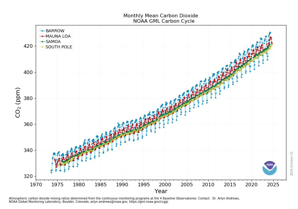
Les mesures modernes pour le taux de CO₂ dans l’atmosphère = [CO₂] débutent en 1958 à Mauna Loa (MLO) et en 1957 à South Pole (SPO). Depuis lors, on constate que le taux de CO₂ dans l’atmosphère augmente : on passe de [CO₂] = 315 ppm (669 Gt-C) en 1959 à 425 ppm (903 Gt-C) en 2025 (1 ppm = 0,0001 % → 2,12 Gt-C → 7,78 Gt-CO₂).
On constate aussi que [CO₂] est plus élevé à MLO qu’à SPO : il est donc préférable d’utiliser une moyenne globale plutôt que les mesures du seul observatoire MLO. Vers 1975, la NOAA dispose de 4 observatoires de référence et peut alors calculer une moyenne globale. Par ailleurs, à la fin des années 70, on dispose des données de température globale mesurée via satellites ainsi que des mesures pour δ¹³C. Pour ces raisons, on utilise ici l’intervalle 1980-2025 afin de disposer des mesures globales les plus fiables.

1.2 La croissance annuelle globale entre 1980 et 2025

La croissance annuelle globale ou Growth rate (ppm/an) est calculée à partir de X(t) = moyenne des observations [CO₂] sur 4 observatoires. La croissance annuelle pour le mois n est obtenue par la différence entre X(t) pour le mois (n+6) avec X(t) pour le mois (n-6), ce qui revient aussi à calculer dX(t)/dt avec dt = 12 mois = 1 an (12 mois afin d’éliminer la saisonnalité).

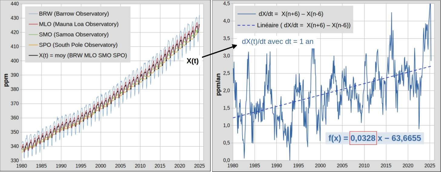
Figure 1 : Le taux de CO₂ global = X(t) = moyenne des 4 observatoires de référence ici (à gauche). dX(t)/dt (croissance annuelle pour le mois n) est calculée par différence entre [CO₂] moyen pour le mois n+6 et le mois n-6 (à droite).

On note que la croissance annuelle globale dX(t)/dt, basée sur la moyenne de 4 observatoires, augmente tendanciellement avec une pente de 0,0328 ppm/an². C’est cette série temporelle de 544 mois entre 1980 et 2025 (fig.1 à droite) qui sera successivement comparée aux émissions anthropiques puis à diverses anomalies de températures.

 
2.  Le flux anthropique (émissions de CO₂ dues à l’homme)

Les émissions anthropiques proviennent de ‘fossil fuel + cement manufacturing’. Le GIEC ajoute un terme secondaire LUC = Land Use Change. Selon Carbonmonitor, il existe une légère modulation saisonnière du flux anthropique.

 
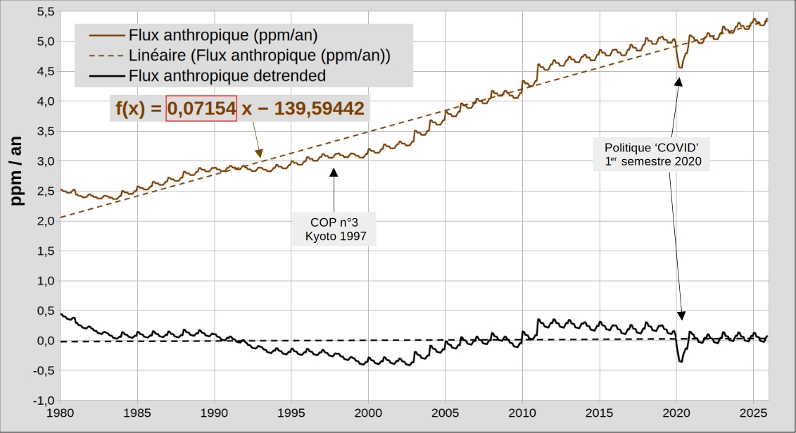
Figure 2 : Flux anthropique (ppm/an) selon CDIAC + BP statistical review + Carbonmonitor. Obtenu par soustraction de la tendance linéaire (pente = 0,07154 ppm/an²), le flux anthropique ‘detrended’ correspond aux écarts avec la tendance (transitoire max au 1^er semestre 2020).

L’action politique semble avoir une influence à la fois modeste et imprévue sur le flux anthropique. Après 1997 (post Kyoto), les tentatives de limitation des émissions se traduisent en pratique par une croissance plus rapide (charbon chinois des années 2000). Lors du 1^er semestre 2020, les effets induits par les politiques ‘Covid’ sont la baisse (éphémère) des émissions et la hausse (moins éphémère) de l’endettement en Europe.

3.  Comparaison de la croissance annuelle avec le flux anthropique

La croissance annuelle du CO2 atmosphérique s’exprime en ppm/an, elle peut donc être comparée directement avec le flux anthropique si on l’exprime en ppm/an (1 ppm/an → 2,12 Gt-C/an → 7,78 Gt-CO₂ /an).
Entre 1980 et 2025, le flux anthropique est environ 2 fois plus grand que la croissance annuelle. Pour satisfaire la thèse du GIEC selon laquelle le flux anthropique est l’unique cause de la croissance annuelle, il est nécessaire de faire un ajustement : multiplier le flux anthropique par le rapport des pentes des tendances long terme. Pour 1980-2025, ce rapport est égal à 0,0328/0,0715 = 46 %. Le GIEC désigne ce rapport par ‘Airborne Fraction’ = AF (pour 1960-2020, AF = 44 %) et en donne la justification suivante : environ la moitié des émissions anthropiques resteraient dans l’atmosphère (mais cela ne s’appliquerait pas aux émissions naturelles!).

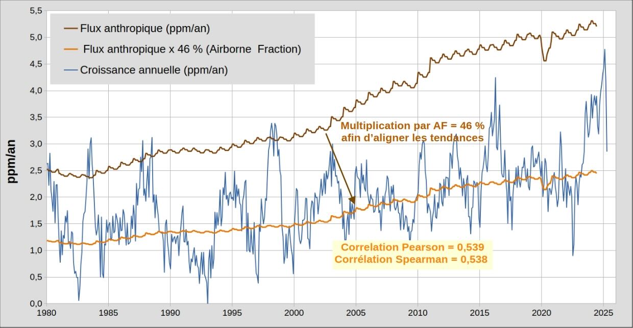
Figure 3a : Comparaison entre la croissance annuelle globale du CO₂ atmosphérique (courbe bleue) et le flux anthropique (courbe marron). Ajustement artificiel (courbe orange) en multipliant par le rapport des 2 pentes = 0,0328/0,0715 = 46 %.

• En pratique, la multiplication du flux anthropique par 46 % revient simplement à aligner artificiellement les 2 tendances.
  On va chiffrer la corrélation qui en résulte, via les corrélations Pearson ou Spearman (0→aucune corrélation, 1→corrélation parfaite). On obtient alors une corrélation apparente Pearson ou Spearman ≈ 0,54 qui est surtout le résultat de l’ajustement artificiel des tendances.
  
• Rigoureusement, la corrélation doit être évaluée en isolant les covariances de court terme (résidus = transitoires = écarts avec les tendances des 2 séries).
  On doit donc soustraire la tendance linéaire (trend) avant comparaison → ‘séries detrended’.

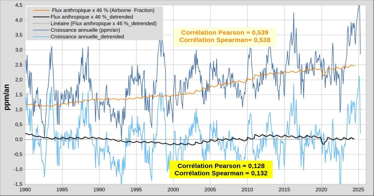
Figure 3b : Comparaison entre flux anthropique multiplié par AF = 46 % (courbe orange) et croissance annuelle (corrélation post ajustement = 0,539 Pearson ou 0,538 Spearman). Comparaison entre les mêmes séries ‘detrended’ → corrélation = 0,128 Pearson ou 0,132 Spearman.

La mauvaise corrélation ≈ 0,13 entre les 2 séries ‘detrended’ indique que la thèse du GIEC doit être remise en question. Sur ce sujet, un lecteur curieux consultera l’article SCE_01/2025 (noter que les observations et périodes utilisées ne sont pas identiques dans les 2 articles).

4.  Comparaison de la croissance annuelle avec UAH_LT

La mauvaise corrélation (≈ 0,13 Pearson ou Spearman) incite à chercher d’autres corrélations avec la croissance du CO₂ dans l’atmosphère. Des scientifiques ont depuis longtemps remarqué la similitude visuelle existant entre croissance annuelle et température. On va donc comparer l’anomalie de température globale dans la basse atmosphère = UAH_LT avec la croissance annuelle du CO₂ atmosphérique = dX(t)/dt.
Mais ces 2 grandeurs ne sont pas de même nature : on doit donc les relier par une expression du type dX(t)/dt ≈a (UAH_LT + b). On utilise ici un coefficient de conversion a (désigné par sensibilité) afin de passer de °C vers ppm/an. Par ailleurs, l’effet de cette sensibilité a est similaire à celui de l’Airborne Fraction du GIEC : ajustement des tendances. Le décalage b n’a pas de signification : on peut avoir b = 0 en changeant la référence de l’anomalie UAH_LT.

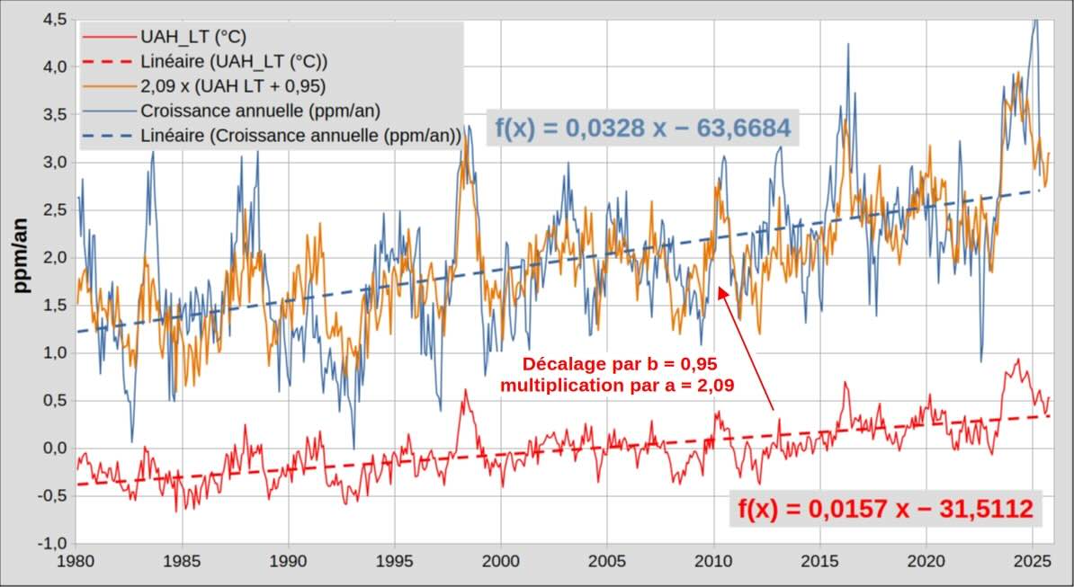
Figure 4a : Comparaison entre les 2 séries : croissance annuelle globale du CO₂ atmosphérique (4 observatoires) et anomalie UAH LT. Ajustement (courbe orange) via le rapport des 2 tendances = sensibilité a = 0,0328/0,0157 =2,09.

La corrélation semble visuellement assez bonne, mais son chiffrage nécessite d’utiliser des séries detrended : c’est-à-dire que l’on doit soustraire les tendances linéaires avant de chiffrer la corrélation.

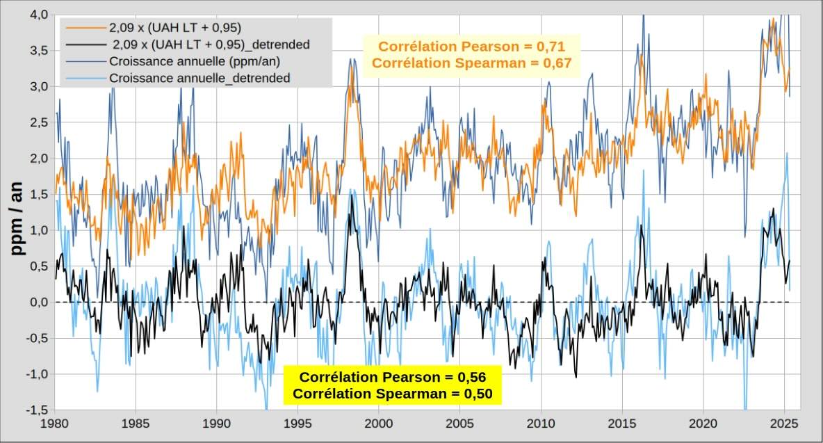
Figure 4b : Comparaison en utilisant la sensibilité a (courbe orange, corrélation post ajustement = 0,71 ou 0,67). Comparaison entre séries ‘detrended’ → corrélation = 0,56 ou 0,50.

La corrélation entre ces 2 séries (0,71 ou 0,67) est plus élevée qu’entre émissions anthropiques et croissance annuelle (0,54, fig.3b) C’est encore plus vrai pour les 2 séries detrended : l’anomalie de température UAH_LT est mieux corrélée (0,56 ou 0,50) avec la croissance annuelle que ne le sont les émissions anthropiques (≈ 0,13).
Les prochains paragraphes s’efforcent de localiser l’origine de cette corrélation entre température et croissance annuelle.

5. Comparaison de la croissance annuelle avec UAH_LT_Tropics

5.1 Anomalie UAH_LT versus anomalie UAH_LT_Tropics

La zone intertropicale (≈ 40 % de la surface du globe qui reçoit ≈ 50 % de la puissance provenant du Soleil) est la zone où la température est la plus élevée. Dans cette zone, la température devrait influencer fortement les échanges naturels de carbone entre les 3 compartiments : Océan, Végétation/sols, Atmosphère (fig.5d). Pour la température on utilise ici l’anomalie UAH_LT_Tropics (Tropics → 20S -20N).

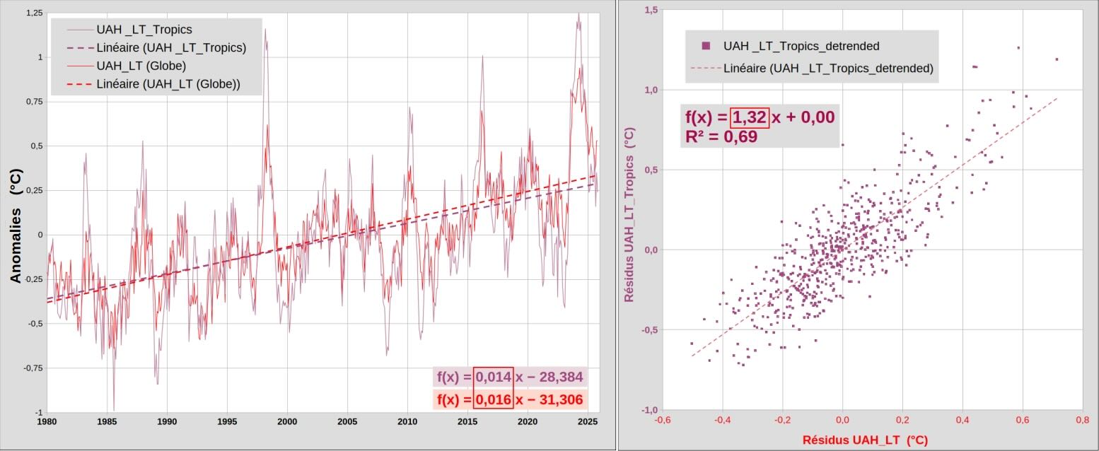
Figure 5a : Deux anomalies de température pour la basse troposphère: globale en rouge et intertropicale en violet. à droite : anomalies en fonction de la date, la globale (0,016 °C/an) croît légèrement plus vite que l’intertropicale (0,014 °C/an). à gauche : Résidus en intertropical (écarts avec la tendance) en fonction des résidus en global : les écarts en intertropical sont ≈ 1,32 fois plus grands que les écarts pour le global.

• La capacité thermique de l’océan est beaucoup plus grande que celle de l’atmosphère : l’océan se réchauffe donc moins vite que l’atmosphère. Pour l’ensemble du globe, l’océan (libre de glace) représente 67 % de la surface, mais pour la zone intertropicale, l’océan représente 75 % de la surface et a donc davantage d’influence. On a ainsi une pente plus faible (0,01415) pour UAH_LT_Tropics que pour UAH_LT (0,01562).

• On note aussi que les transitoires ou écarts avec la tendance sont plus grands (x 1,32) pour la zone intertropicale : ces transitoires sont souvent liés à des événements ENSO (El Niño et La Niña ) originaires de l’océan Pacifique intertropical.

5.2 Comparaison anomalie UAH_LT_Tropics et croissance annuelle

• Pour la croissance annuelle du CO₂ dans la zone intertropicale, on utilise la moyenne des 2 observatoires MLO et SMO.
  La tendance de la croissance annuelle MLO SMO (0,0329) reste quasi inchangée par rapport à celle de 4 observatoires (0,0328). La corrélation dans la zone intertropicale est-elle meilleure que celle pour l’ensemble du globe (fig. 4b)? 

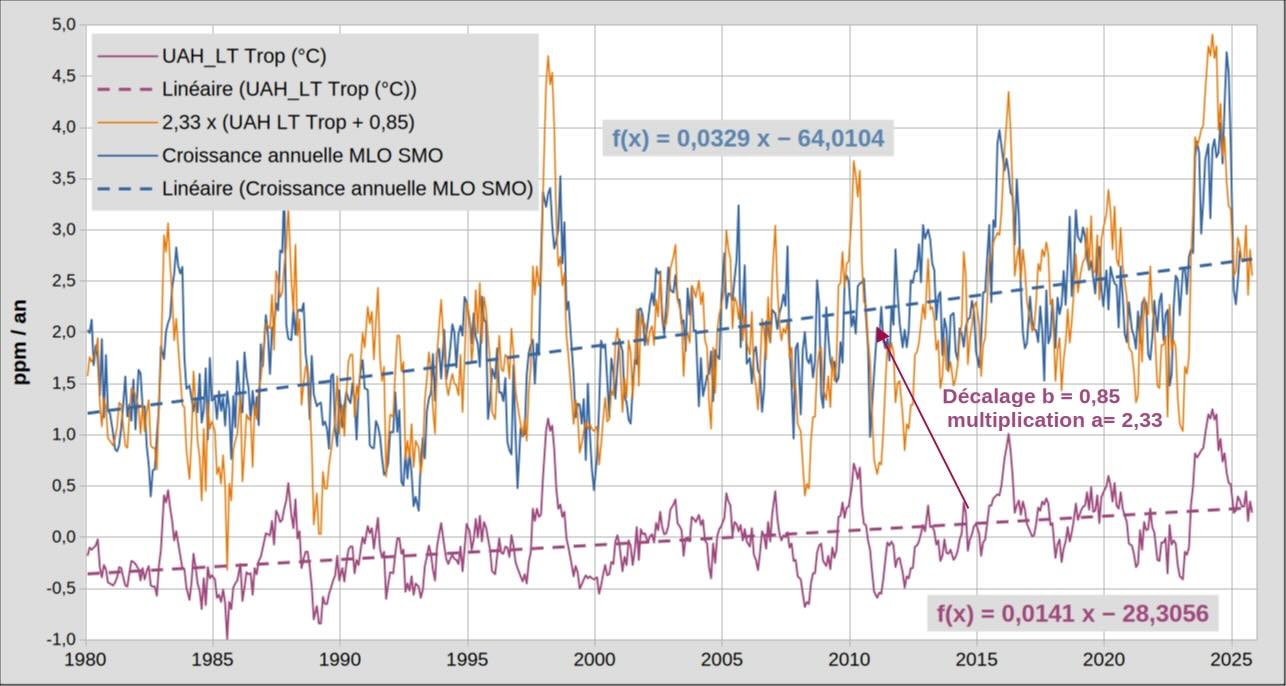
Figure 5b : Croissance annuelle du CO₂ atmosphérique (moyenne MLO SMO) et anomalie UAH_LT_Tropics (courbe violette). Ajustement UAH_LT_Tropics (courbe orange) via le rapport des 2 tendances = sensibilité a = 0,0329 / 0,0141 = 2,33.

– Selon les archives glaciaires, il existerait un décalage ≈ 800 ans entre le proxy [CO₂] et le proxy température : les variations du proxy température précèdent les variations du proxy [CO₂].
– Selon Humlum et al 2013, il existerait un retard systématique ≈ 10 mois entre d[CO₂] /dt = croissance annuelle et la température. Mais les meilleures observations modernes (fig.5b) indiquent plutôt une quasi-simultanéité (à ± 5 mois) entre les pics croissance annuelle. intertropicale (MLO SMO) et température intertropicale via satellites.
Comme précédemment, on doit chiffrer la corrélation à partir des séries detrended.

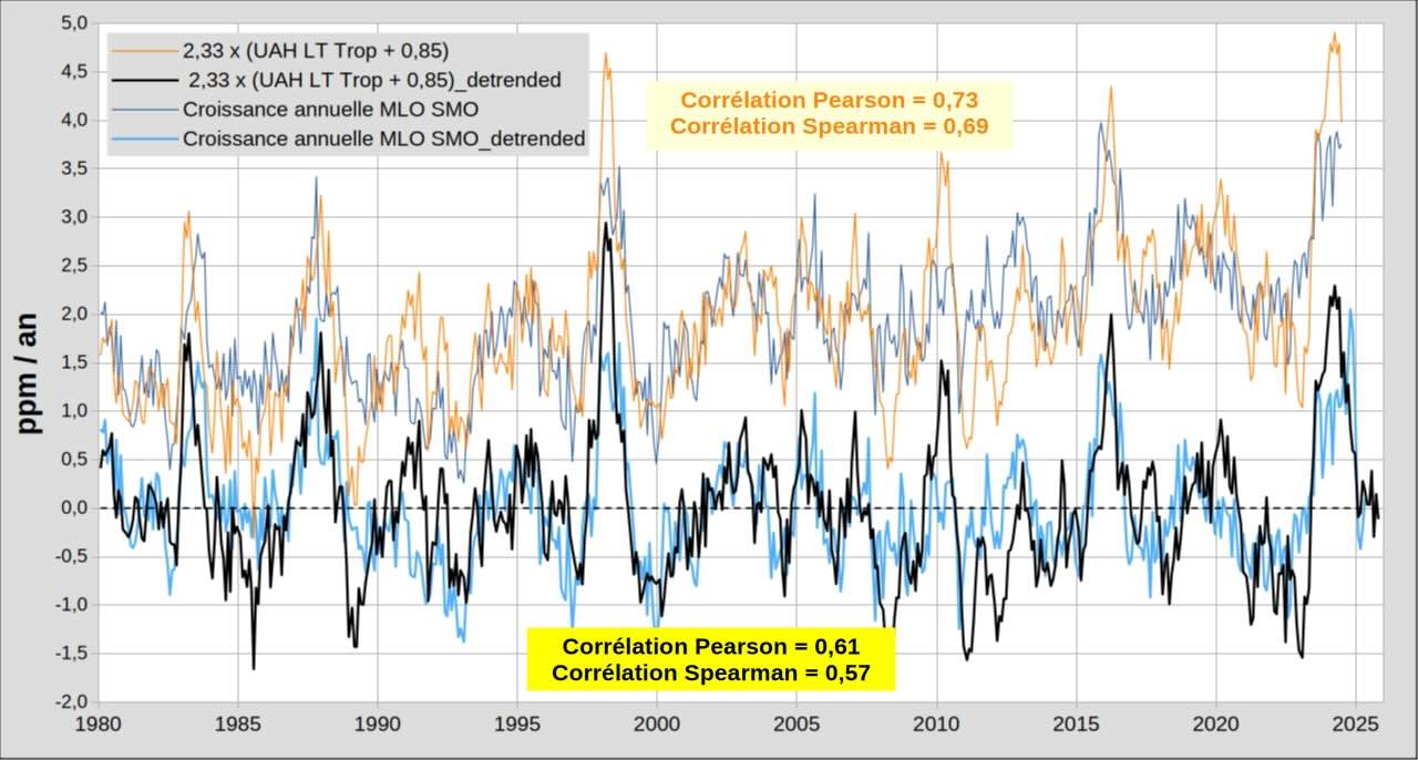
Figure 5c : Comparaison après ajustement (courbe orange) via sensibilité a = 2,33  (corrélation post ajustement = 0,73 ou 0,69). Comparaison entre séries ‘detrended’→ corrélation =0,61 ou 0,57.

 La corrélation est meilleure avec UAH_TL_Tropics_detrended (0,61 ou 0,57) qu’avec UAHLT_detrended (0,56 ou 0,50 fig. 4b). Quelles sont les raisons qui permettraient à la température dans la zone intertropicale d’être corrélée avec la croissance annuelle ? La température intertropicale n’influence pas les émissions anthropiques, en revanche, elle peut influencer les échanges de carbone naturels entre l’atmosphère et les compartiments océan ou végétation/sols (flux 1 2 3 4 fig. 5d). Le flux 1 (correspondant au dégazage de carbone par l’océan intertropical) dépend beaucoup de la température.

Figure 5d : à gauche, schéma simplifié des échanges de carbone avec 4 flux naturels + flux anthropique
à droite, le tableau montre que c’est en zone intertropicale que croissance annuelle et température sont le mieux corrélées (0,61 ou 0,57).

6.  Tendances (long terme) versus transitoires (court terme)

La figure ci-dessous, en utilisant les outils classiques de comparaison entre séries temporelles (544 résidus en XY), donne un autre argument pour choisir une thèse privilégiant UAH_LT_Tropics plutôt que la thèse du GIEC.

 
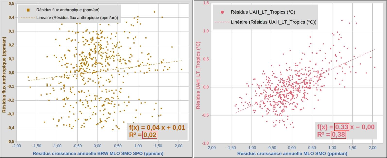
Figure 6a : à gauche, la thèse du GIEC est contredite par l’absence de relation entre résidus ou transitoires (R² = 0,02). A droite, le relatif alignement des résidus (R² = 0,38) permet de soupçonner une relation entre résidus des 2 séries.

6.1 Croissance annuelle : le long terme et les transitoires

• Pour la croissance annuelle, les rédacteurs du GIEC (AR6 § 5.21) séparent la tendance de long terme (qui serait la conséquence du seul flux anthropique) et les transitoires de court terme (les flux 3 et 4 seraient influencés par ENSO).

• On note que le rapport liant les résidus ou transitoires (0,33 →fig.6a à droite) est proche de celui liant les tendances (0,43 = 0,0141/0,0329 → fig.5b). Le physicien qui n’est pas rédacteur du GIEC y voit un indice que les mêmes phénomènes physiques commandent la tendance et les transitoires. Pour aller au-delà, on doit tenir compte du bruit aléatoire qui affecte toute observation. Pour un même niveau de bruit aléatoire, les grands écarts (transitoires) avec la tendance sont moins affectés que les petits écarts. Si on ne conserve que les résidus correspondant aux plus grands écarts avec les tendances, alors on améliore le rapport signal/bruit.
  Afin de retenir ≈ 50 % des 544 résidus initiaux, on ne conserve que les écarts (résidus) > à 0,15 ppm/an ou > à 0,15 °C.

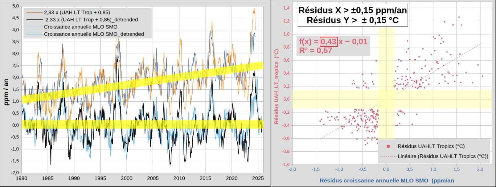
Figure 6b : à gauche idem fig.5c mais les bandes jaunes montrent les écarts (résidus) à éliminer afin de conserver ≈ 50 % des écarts (résidus) ; à droite, idem fig.6a droite mais en ne conservant que ≈ 50 % des résidus (les plus grands écarts).

• En conservant les écarts (transitoires ou résidus) les plus grands (≈ 50 % des transitoires), on constate que le rapport (0,43) liant les écarts (transitoires ou résidus) les plus grands est désormais le même que celui liant les tendances de long terme (0,43). Ce résultat est obtenu avec une procédure classique en traitement du signal et en utilisant les meilleures observations disponibles pour la zone intertropicale. Ce résultat important est explicité ci-dessous.
  – Une hausse de long terme de 0,43 °C pour UAH_LT_Tropics coïncide avec une augmentation de long terme de 1 ppm/an pour la croissance annuelle.
  – Une hausse transitoire de 0,43 °C (écarts > 0,15 °C pour UAH_LT_Tropics) coïncide aussi avec une augmentation transitoire de 1 ppm/an pour la croissance annuelle.
  
• En zone intertropicale, le rapport (Δ température) / (Δ croissance annuelle) = 0,43 °C/ppm/an est identique pour le long terme et pour les transitoires les plus grands. Les 2 paragraphes suivants montrent que l’onne retrouve pas cette similitude entre long terme et transitoires pour UAH_LT ou pour le flux anthropique. 

6.2 Température globale (UAH LT) ou intertropicale (UAH LT Tropics)?

La figure ci-dessous montre que l’anomalie de température UAH_LT ne présente pas cette similitude entre long terme et transitoires. Le rapport des tendances est 0,01572 / 0,0328 = 0,48 (fig. 4a), mais en comparant 100 % des résidus, le rapport = 0,18 et pour les résidus les plus grands (50%) le rapport = 0,23.

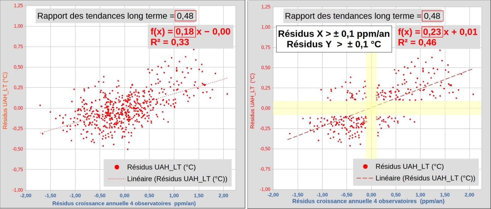
Figure 6c : à gauche, comparaison pour 100 % des résidus ; à droite, comparaison pour 50 % des résidus : leur rapport = 0,23 reste éloigné du rapport des tendances long terme = 0,48.

6.3 La thèse du GIEC n’est pas compatible avec les observations

• Pour la croissance annuelle, les rédacteurs du GIEC (AR6 § 5.21) séparent donc les transitoires de court terme (qui seraient pilotés par ENSO via les flux 3 et 4) et la tendance de long terme qui serait la conséquence du seul flux anthropique (le GIEC multiplie par le rapport des tendances = 46 % désigné par Airborne Fraction, voir fig. 3a)..

• On rappelle le résultat obtenu en comparant, après ajustement, le flux anthropique et la croissance du CO₂ atmosphérique : corrélation Pearson 0,54 contre 0,73 pour UAH_LT_Tropics. Pour les mêmes séries detrended on a0,13 contre 0,61 ou 0,57 pour UAH_LT_Tropics. On reprend la procédure illustrée à la fig. 6c, mais en l’appliquant au flux anthropique : retrouve-t-on le rapport des tendances long terme (0,07154/0,0328 = 2,18) en faisant le rapport des résidus (écarts ou transitoires) ?

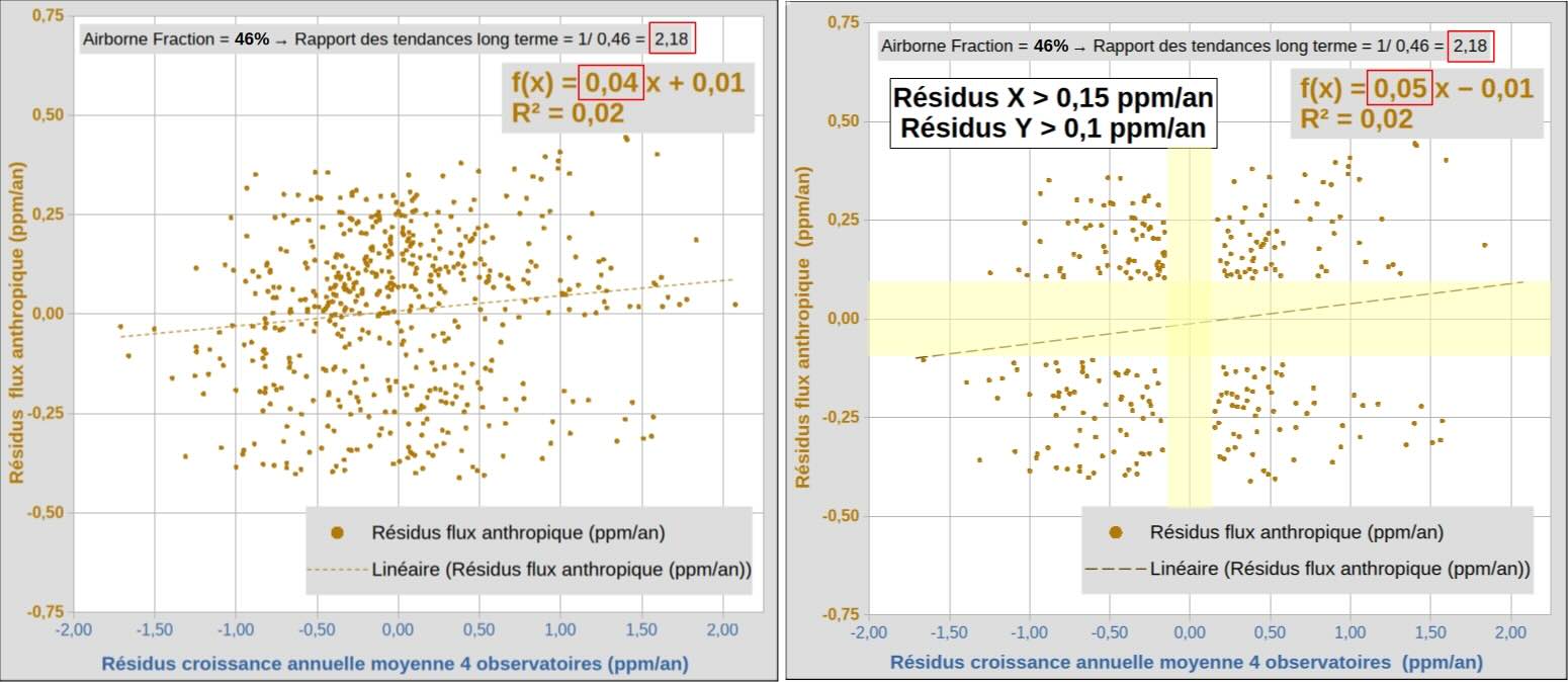
Figure 6d : Deux tracés des résidus du flux anthropique en fonction des résidus de la croissance annuelle.
A gauche, on utilise 100 % des résidus ; à droite, on ne conserve que 50 % des résidus (les plus grands).

• Aucune similitude n’existe entre le rapport des tendances de long terme (2,18) et le rapport des transitoires (0,04), même en sélectionnant les plus grands (0,05).
  Aucune relation n’existe (R² = 0,02) entre transitoires de la croissance annuelle et transitoires du flux anthropique.
  La corrélation n’implique pas toujours la causalité mais en revanche l’absence de corrélation indique une absence de causalité.

• Le tableau ci-dessous résume l’analyse des corrélations avec la croissance annuelle du CO₂ atmosphérique. L’analyse n’utilise pas la notion de durée de séjour mais uniquement les meilleures observations (544 mois entre 1980 et 2025).

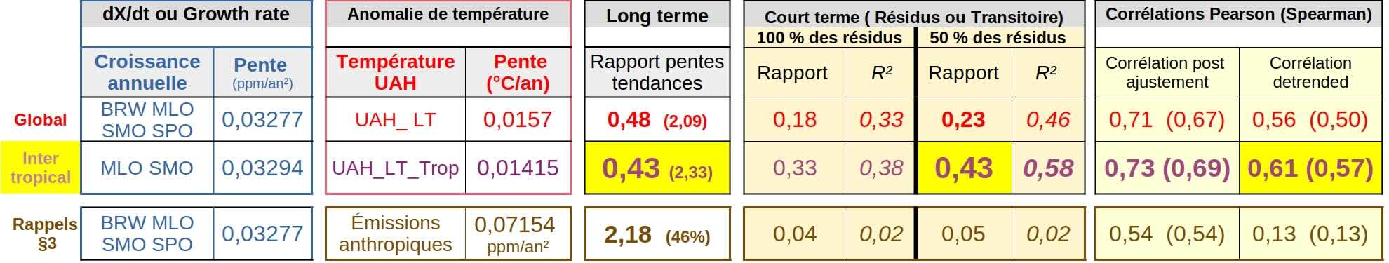
Figure 6e : Tableau récapitulatif des comparaisons ; la température en intertropical UAH_LT_Trop présente la meilleure corrélation detrended (0,61 ou 0,57) et les rapports Δ température/Δ croissance sont identiques (0,43) pour le long terme et les grands transitoires.

La cause principale de la croissance du CO₂ atmosphérique ne semble donc pas être le flux anthropique, la cause principale semble liée aux diverses températures en zone intertropicale.

Le paragraphe qui suit donne les raisons supplémentaires pour lesquelles ‘Revisiting the carbon cycle’ privilégie finalement la température en surface de l’océan intertropical (SSTi) et le flux 1 (fig.5d).

7.  Le dégazage océanique intertropical serait la cause majeure de la corrélation

7.1 Les ordres de grandeurs

La surface du globe entre 23°26’ S et 23°26’ N est à 75 % océanique → la température de la basse troposphère en zone intertropicale est largement le reflet de la température de l’océan SSTi = Sea Surface Temperature intertropicale. En effet, la capacité thermique est plus élevée pour l’océan que pour l’atmosphère (selon la profondeur, le rapport est 10 à 1000 ici fig.1).
– Le stock de carbone dans l’océan est environ 16 fois plus grand que celui dans Végétation/sols.
– La pression partielle pour le CO₂ dans l’eau à la surface de l’océan varie très fortement selon sa température (fonction de SST^12,5). Une même augmentation de température SST aura donc plus d’effet sur le flux 1 (zone intertropicale chaude SST ≈ 25 °C à 32 °C) que sur le flux 2 (hautes latitudes, zone froide SST ≈ 5°C à 15°C ). Pour une même augmentation de 0,5°C, le lecteur peut vérifier que  30,5^12,5  – 30^12,5  >  10,5^12,5 – 10^12,5  (le calcul correct en kelvin obtient la même inégalité).

7.2 L’isotope ¹³C et δ¹³C

• Aux considérations précédentes, ‘Revisiting the carbon cycle’ ajoute les observations modernes sur l’isotope ¹³C dans l’atmosphère : l’évolution de δ¹³C ne peut provenir uniquement d’un apport net de carbone anthropique (voir §4 ici ).
  Un apport net complémentaire est nécessaire : provient-il du compartiment Océan ou bien du compartiment Végétation/sols ?

• A propos du compartiment Végétation/sols, il est vraisemblable que la décomposition végétale (flux 3 de la fig.5d) augmente avec la température. Néanmoins, la décomposition végétale est probablement inférieure à l’absorption de carbone par la végétation (flux 4 de la fig. 5d) car le verdissement global de la planète laisse penser que flux 4 > flux 3 → pas d’apport net.

• Une même augmentation de température a plus d’effet sur le flux 1 (zone chaude) que sur le flux 2 (zone froide) → flux 1 > flux 2 → apport net possible. D’autre part, pour le flux 1 en zone intertropicale, δ¹³C est inférieur de 1,5 ‰ à celui de l’atmosphère (fig.8 ici). Un apport net complémentaire de carbone depuis l’océan intertropical vers l’atmosphère équilibrerait alors le bilan pour δ¹³C (‘Revisiting the carbon cycle’ estime le flux 1 en sorte de fermer le bilan pour δ¹³C).

• ‘Revisiting the carbon cycle’ compare donc la croissance annuelle (mais observée à MLO) et la température de l’océan intertropical SSTi (mais depuis 1959, donc hors observations satellites). Dans sa figure 2, on défalque de la croissance annuelle la faible part anthropique : la corrélation est alors excellente. Dans sa figure 3 (similaire à la figure 5b ici), on défalque aussi la part anthropique. Au § 7 et dans les figures 22,23 et 24, on détaille l’évolution 1980-2020 de δ¹³C.

8. Conclusions

• Le modèle utilisé dans « Revisiting the carbon cycle » s’appuie sur l’analyse des corrélations basées sur les mesures modernes les plus fiables. La faible corrélation entre le flux anthropique ajusté via ‘airborne fraction’ et la croissance annuelle remet en question la thèse du GIEC. En revanche, la corrélation observée entre les séries detrended suggère que la température de la zone intertropicale influence significativement la croissance annuelle, principalement via les échanges naturels de carbone (fig. 6e).

• Concernant les échanges naturels de carbone dans la zone intertropicale, d’autres éléments (§7) indiquent que l’influence de l’océan prédomine sur celle de la végétation et des sols. Cependant, la corrélation obtenue n’est pas parfaite : l’océan jouerait un rôle majeur, mais d’autres facteurs secondaires interviendraient également.

• Dans les sciences de la nature, il est courant de quantifier les corrélations en sélectionnant les meilleures observations disponibles et en appliquant des méthodes de traitement du signal. Bien que la jeune science du climat soit souvent considérée comme ‘settled’, pourquoi ne pas lui appliquer ces méthodes éprouvées ?

• Dans le rapport AR6 WG1 du GIEC, le terme « model » apparaît 14 192 fois, contre 3 106 occurrences pour le terme « observation » (82 % vs 18%). Si le bureau du GIEC reconnaissait que les observations doivent guider les modèles, il sélectionnerait alors davantage d’observateurs parmi ses rédacteurs. Malheureusement, un tel aggiornamento risquerait de fragiliser le ‘consensus scientifique’ des modélisateurs/rédacteurs.

La partie 2 de l’article présente le modèle utilisé dans les figures 14 et 15 du § 6 de ‘Revisiting the carbon cycle’.
La partie 3 propose des illustrations permettant de mieux appréhender le modèle et fournit des réponses aux objections courantes.

Références

Revisiting The Carbon Cycle  https://doi.org/10.53234/scc202510/10

[CO₂] selon NOAA  Observatoires de référence  
UAH LT et LT_Tropics  https://www.nsstc.uah.edu/data/msu/v6.1/tlt/uahncdc_lt_6.1.txt
Émissions anthropiques selon CDIAC
Émissions anthropiques selon BP statistical review
Émissions anthropiques selon Carbonmonitor.
SST selon NOAA   https://www.psl.noaa.gov/data/gridded/data.noaa.oisst.v2.highres.html
KNMI Climate explorer  https://climexp.knmi.nl

Le cycle du carbone (Camille Veyres 2024)
The Rational Climate e-Book(section 1.4 page 32) de Patrice Poye
Une comparaison absente du rapport du GIEC SCE_01/2025
Addendum.pdf

---

Revisiting the carbon cycle

1/3 Modern observations guide the model

par J.C. Maurin, Professeur agrégé de physique

In 2025, the peer-reviewed scientific journal Science of Climate Change published a 50-page study entitled “Revisiting the carbon cycle.” This work thoroughly challenges the carbon cycle models proposed by the IPCC. We will detail the new model presented in this publication in three parts:
1. Modern observations guide the model;
2. Introduction to the MPO model;
3. Additions, illustrations, responses to objections.
Since the 1990s, under the influence of the UN/IPCC, one hypothesis has become the consensus: the increase in atmospheric CO₂ is solely due to human activities. Conversely, this first part of the article puts forward arguments suggesting that this increase is mainly linked to temperatures in tropical regions. The article is available here in PDF format.

1. Atmospheric CO₂ and its annual growth

1.1 Selecting the most reliable overall observations

Modern measurements of atmospheric CO₂ levels = [CO₂] began in 1958 at Mauna Loa (MLO) and in 1957 at South Pole (SPO). Since then, the level of CO₂ in the atmosphere has been increasing: from [CO₂] = 315 ppm (669 Gt-C) in 1959 to 425 ppm (903 Gt-C) in 2025 (1 ppm = 0.0001% → 2.12 Gt-C → 7.78 Gt-CO₂) .
It has also been observed that [CO₂] is higher at MLO than at SPO: it is therefore preferable to use an overall average rather than measurements from the MLO observatory alone. Around 1975, NOAA had four reference observatories and was able to calculate a global average. Furthermore, at the end of the 1970s, global “temperature” data measured via satellites became available, as well as measurements for δ¹³C.
For these reasons, the 1980-2025 interval is used to obtain the most reliable global measurements possible.

1.2 Global annual growth between 1980 and 2025

The overall annual growth rate (ppm/year) is calculated from X(t) = average of [CO₂] observations at four observatories. The annual growth for month n is obtained by the difference between X(t) for month (n+6) and X(t) for month (n-6), which also corresponds to calculating dX(t)/dt with dt = 12 months = 1 year (12 months to eliminate seasonality).

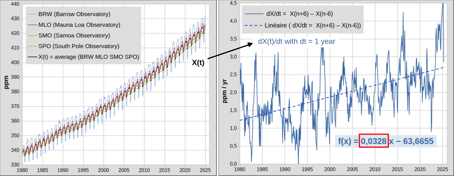
Figure 1: Global CO₂ level = X(t) = average of the four reference observatories here (left).
dX(t)/dt (annual growth for month n) is calculated as the difference between the average [CO₂] for month n+6 and month n-6 (right).

It should be noted that the global annual growth dX(t)/dt based on the average of 4 observatories, tends to increase at a rate of 0.0328 ppm/year². It is this time series of 544 months between 1980 and 2025 (Fig. 1, right) that will be successively compared to anthropogenic emissions and then to various temperature anomalies.

2. Anthropogenic flux (CO₂ emissions caused by humans)

Anthropogenic emissions come from fossil fuel and cement manufacturing. The IPCC adds a secondary term, LUC = Land Use Change. According to Carbonmonitor, there is a slight seasonal modulation in anthropogenic flux.

 
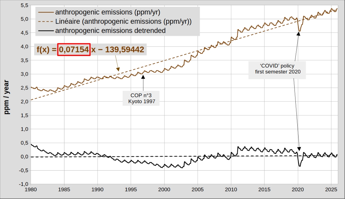
Figure 2: Anthropogenic flux (ppm/year) according to CDIAC + BP statistical review + Carbonmonitor. Obtained by subtracting the linear trend (slope = 0.07154 ppm/year²), the detrended anthropogenic flux also corresponds to deviations from the trend (maximum transient in the first half of 2020).

Political action seems to have a modest and unexpected influence on anthropogenic flux. After 1997 (post-Kyoto), attempts to limit emissions result in faster growth in practice (Chinese coal in the 2000s). In the first half of 2020, the effects of Covid policies were a (short-lived) decline in emissions and a (less short-lived) increase in debt in Europe.

3. Comparison of annual growth with anthropogenic flux

The annual growth of atmospheric CO₂ is expressed in ppm/year, so it can be directly compared with anthropogenic flux if expressed in ppm/year (1 ppm/year → 2.12 Gt-C/year → 7.78 Gt-CO₂/year).
Between 1980 and 2025, the anthropogenic flux is approximately twice as large as the annual growth. To satisfy the IPCC’s thesis that anthropogenic flux is the sole cause of annual growth, an adjustment must be made: multiply the anthropogenic flux by the ratio of the slopes of the long-term trends. For 1980-2025, this ratio is equal to 0.0328/0.0715 = 46%.
The IPCC refers to this ratio as the “Airborne Fraction” = AF (for 1960-2020, AF = 44%) and gives the following justification: approximately half of anthropogenic emissions remain in the atmosphere (but this does not apply to natural emissions!).

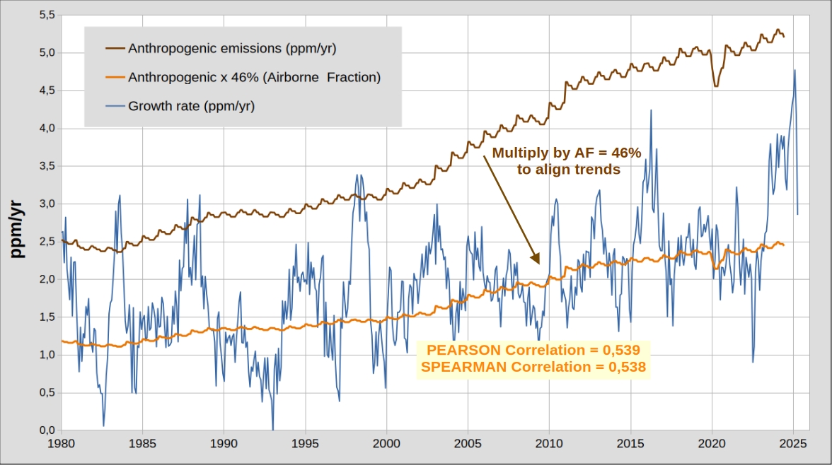
Figure 3a: Comparison between the overall annual growth in atmospheric CO₂ (blue curve) and anthropogenic flux (brown curve). Artificial adjustment (orange curve) by multiplying by the ratio of the two slopes (Figs. 1 and 2) 0.0328/0.0715 = 46%.

• In practice, multiplying the anthropogenic flux by 46% simply amounts to artificially aligning the two trends.
  We will quantify the resulting correlation using the PEARSON correlation or SPEARMAN correlation (0→no correlation, 1→perfect correlation). This gives us an apparent correlation PEARSON or SPEARMAN = 0.54, which is mainly the result of the artificial adjustment of the trends.
  
•  Strictly speaking, the correlation must be evaluated by isolating the short-term covariances (residuals = transients = deviations from the trends of the two series). We must therefore subtract the linear trend before comparison → ‘detrended series’.

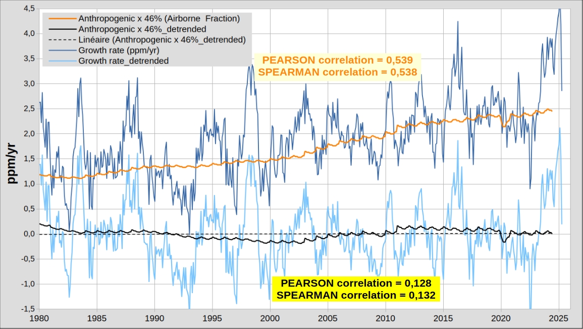
Figure 3b: Comparison between anthropogenic flux multiplied by AF = 46% (orange curve) and annual growth (post-adjustment correlation = 0.539 Pearson or 0.538 Spearman). Comparison between the same detrended series → correlation = 0.128 Pearson or 0.132 Spearman.

The poor correlation ≈ 0.13 between the two detrended series indicates that the IPCC’s thesis should be questioned. On this subject, interested readers may consult article SCE_01/2025 (note that the observations and periods used are not identical in the two articles).

4. Comparison of annual growth with UAH_LT

The poor correlation (≈ 0.13 Pearson or Spearman) encourages us to look for other correlations with the growth of CO₂ in the atmosphere. Scientists have long noticed the visual similarity between annual growth and temperature. We will therefore compare the global temperature anomaly in the lower atmosphere = UAH_LT with the annual growth of atmospheric CO₂ = dX(t)/dt. However, these two quantities are not of the same nature: we must therefore link them using an expression of the type dX(t)/dt ≈ a (UAH_LT + b). Here we use a conversion coefficient a (referred to as sensitivity) to convert from °C to ppm/year. Furthermore, the effect of this sensitivity a is similar to that of the IPCC’s Airborne Fraction: adjustment of trends. The offset b has no significance: we can have b = 0 by changing the reference for the UAH_LT anomaly.

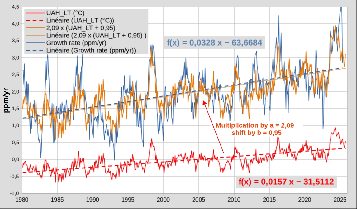
Figure 4a: Comparison between the two series: overall annual growth in atmospheric CO₂ (four observatories) and UAH LT anomaly. Adjustment (orange curve) via the ratio of the two trends = sensitivity a = 0.0328 / 0.0157 = 2.09.

The correlation seems visually quite good, but its quantification requires the use of detrended series: that is, the linear trends must be subtracted before quantifying the correlation.

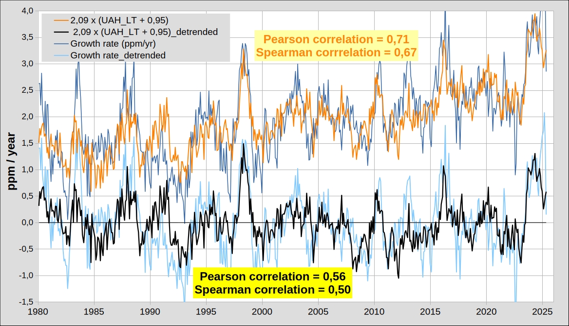
Figure 4b: Comparison using sensitivity a (orange curve, post-adjustment correlation = 0.71 or 0.67). Comparison between detrended series → correlation = 0.56 or 0.50.

The correlation between these two series (0.71 or 0.67) is higher than between anthropogenic emissions and annual growth (0.54, Fig. 3b). This is even more true for the two detrended series: the UAH_LT temperature anomaly correlates better (0.56 or 0.50) with annual growth than anthropogenic emissions do (≈ 0.13).
The following paragraphs attempt to locate the origin of this correlation between temperature and annual growth.

5. Comparison of annual growth with UAH_LT_Tropics

5.1 UAH_LT anomaly versus UAH_LT_Tropics anomaly

The intertropical zone (≈ 40% of the Earth’s surface and ≈ 50% of the energy from the Sun) is the area where the temperature is highest. In this zone, temperature should therefore have a strong influence on natural carbon exchanges between the three compartments: Ocean, Vegetation/Soil, and atmosphere (Fig. 5d). For temperature, we use the UAH_LT_Tropics anomaly (Tropics → 20S -20N).

Figure 5a: Two UAH temperature anomalies for the lower troposphere: global in red and intertropical in purple. Right: anomalies as a function of date; the global anomaly (0.016 °C/year) is increasing slightly faster than the intertropical anomaly (0.014 °C/year). Left: Residuals for the intertropical region (deviations from the trend) as a function of residuals for the global region: deviations in the intertropical region are ≈ 1.32 times greater than deviations for the global region.

• The heat capacity of the ocean is much greater than that of the atmosphere: the ocean therefore warms less quickly than the atmosphere. For the globe as a whole, the ocean (free of ice) represents 67% of the surface area, but for the intertropical zone, the ocean represents 75% of the surface area and therefore has a greater influence. This results in a lower slope (0.01415) for UAH_LT_Tropics than for UAH_LT (0.01562).

• It should also be noted that transients or deviations from the trend are greater (x 1.32) for the intertropical zone: these transients are often linked to ENSO events (El Niño and La Niña) originating in the intertropical Pacific Ocean.

5.2 Comparison of UAH_LT_Tropics anomaly and annual growth

• For annual growth rate in the intertropical zone, we use the average from the two observatories, MLO and SMO. The MLO SMO annual growth trend (0.0329) remains virtually unchanged from that for four observatories (0.0328). Is the correlation in the intertropical zone better than that for the globe as a whole (Fig. 4b)?

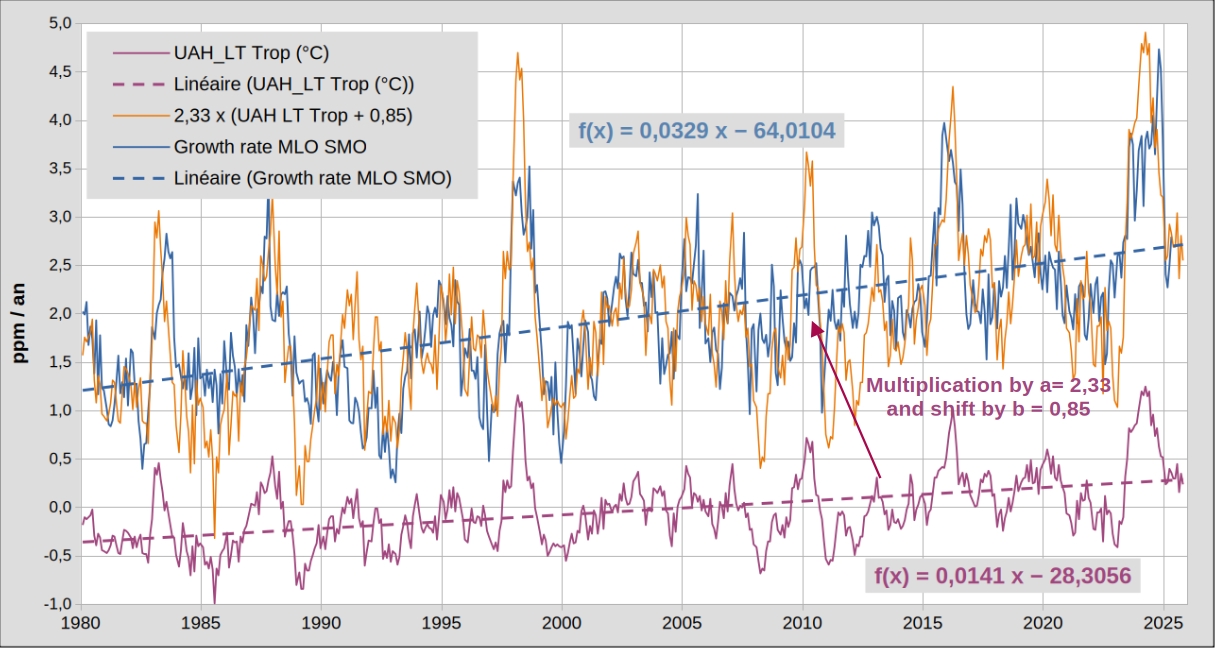
Figure 5b: Annual growth in atmospheric CO₂ (MLO SMO average) and UAH_LT_Tropics anomaly (purple curve). Adjustment of UAH_LT_Tropics (orange curve) via the ratio of the two trends = sensitivity a = 0.0329 / 0.0141 = 2.33.

– According to ice core records, there is an ≈ 800-year lag between the [CO₂] proxy and the temperature proxy (variations in the temperature proxy precede variations in the [CO₂] proxy).
– According to Humlum et al 2013, there is a systematic delay of ≈ 10 months between d[CO₂] /dt = annual growth and temperature. However, the best modern observations (Fig. 5b) indicate instead a near-simultaneity (to ± 5 months) between the intertropical annual growth peaks (MLO SMO) and intertropical temperature via satellites.
As before, the correlation must be calculated from the detrended series.

 
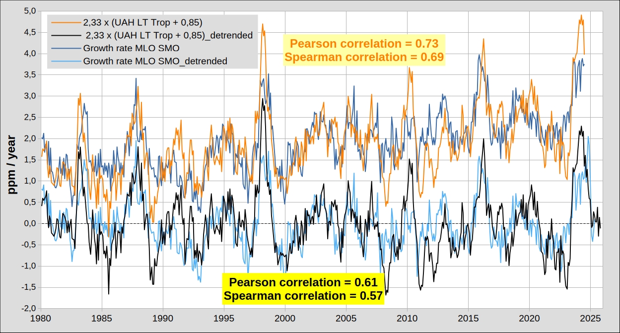
Figure 5c: Comparison after adjustment (orange curve) via sensitivity a = 2.33 (post-adjustment correlation = 0.73 or 0.69). Comparison between detrended series → correlation = 0.61 or 0.57.

The correlation is better with UAH_TL_Tropics_detrended (0.61 or 0.57) than with UAHLT_detrended (0.56 or 0.50 fig. 4b). What are the reasons that would allow the temperature in the intertropical zone to be correlated with annual growth? Intertropical temperature does not influence anthropogenic emissions, but it can influence natural carbon exchanges between the atmosphere and the ocean or vegetation/soil compartments (flows 1, 2, 3, 4, Fig. 5d). Flow 1 (corresponding to carbon degassing by the intertropical ocean) is highly dependent on temperature.

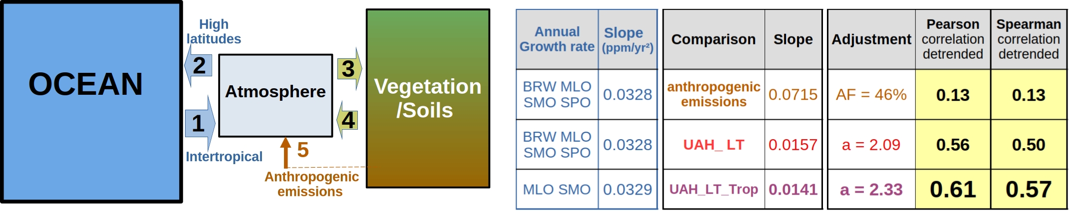
Figure 5d: on the left, simplified diagram of carbon exchanges with four natural flows + anthropogenic flow. On the right, the table shows that annual growth and temperature are most closely correlated (0.61 or 0.57) in the intertropical zone.

6. Trends (long term) versus transiznts (short term)

• The figure below, using standard tools for comparing time series (544 residuals in XY), provides another argument for choosing a thesis favoring UAH_LT_Tropics rather than the IPCC thesis.

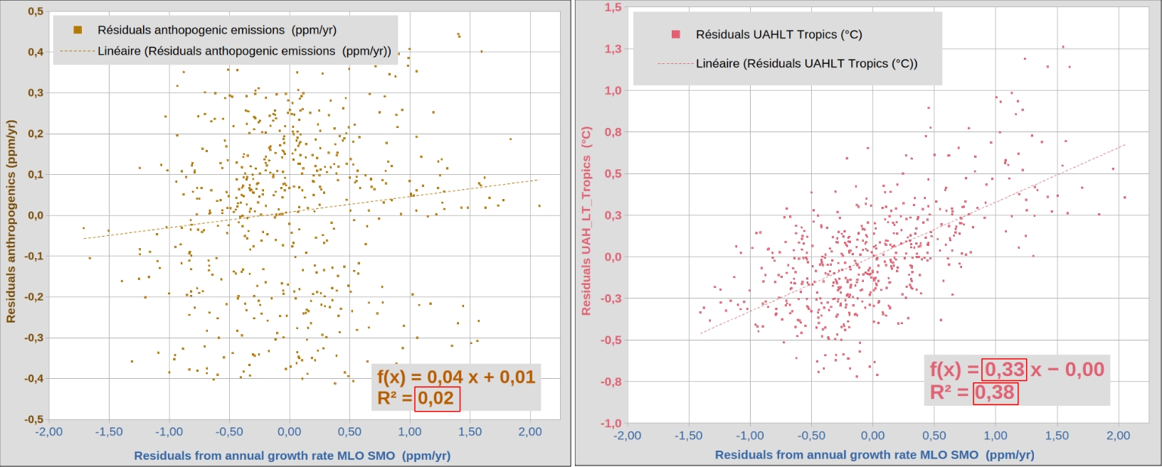
Figure 6a: on the left, the IPCC’s thesis is contradicted by the absence of a relationship between residuals/transients (R² = 0.02). On the right, the relative alignment of the residuals (R² = 0.38) suggests a relationship between the residuals of the two series.

6.1 Annual growth: long term and transients

• For annual growth, the IPCC authors (AR6 § 5.21) separate the long-term trend (which would be the result of anthropogenic flux alone) from short-term transients (fluxes 3 and 4 would be influenced by ENSO).

• It should be noted that the ratio linking the residuals or transients (0.33 → Fig. 6a on the right) is close to that linking the trends (0.43 = 0.0141/0.0329 → Fig. 5b). Physicists who are not IPCC authors see this as an indication that the same physical phenomena govern both the trend and the transients. To go further, we must take into account the random noise that affects all observations. For the same level of random noise, large deviations (transients) from the trend are less affected than small deviations. If we retain only the residuals corresponding to the largest deviations from the trends, then we improve the signal-to-noise ratio .
In order to retain ≈ 50% of the initial 544 residuals, only deviations (residuals) > 0.15 ppm/year or > 0.15 °C are retained.

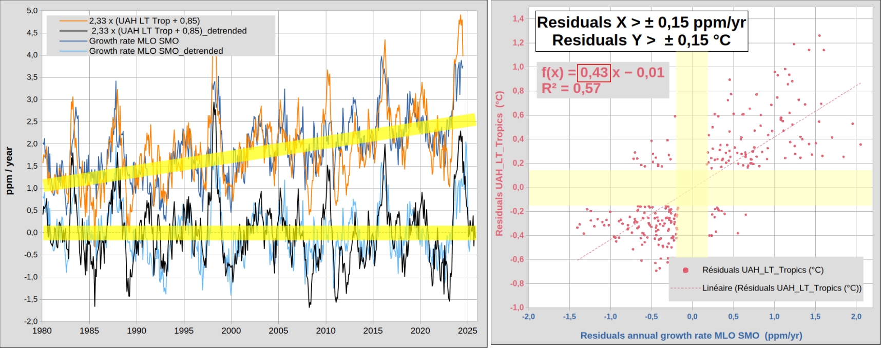
Figure 6b: on the left, same as fig. 5c, but the yellow bands show the deviations/residuals to be eliminated in order to retain ≈ 50% of the deviations/residuals. On the right, same as fig. 6a on the right, but retaining only ≈ 50% of the residuals (the largest deviations).

• By retaining the largest deviations/transients/residuals (≈ 50% of transients), we note that the ratio (0.43) linking the largest deviations (transitory or residual) is now the same as that linking long-term trends (0.43). This result is obtained using a standard signal processing procedure and the best observations available for the intertropical zone.
This important result is explained below.

• – A long-term increase of 0.43°C for UAH_LT_Tropics coincides with a long-term increase of 1 ppm/year for annual growth.
– A transient increase of 0.43°C (deviations > 0.15°C for UAH_LT_Tropics) also coincides with a transient increase of 1 ppm/year for annual growth.

• In the intertropical zone, the ratio (Δ temperature)/(Δ annual growth) = 0.43 °C/ppm/year is identical for the long term and for the largest transients. The following two paragraphs show that this similarity between the long term and transients is not found for UAH_LT or for anthropogenic flux.

6.2 Global (UAH _LT) or intertropical (UAH _LT_ Tropics)?

The figure below shows that the UAH_LT temperature anomaly does not exhibit this similarity between long-term and transient trends. The trend ratio is 0.01572 / 0.0328 = 0.48 (Fig. 4a), but when comparing 100% of the residuals, the ratio = 0.18, and for the largest residuals (50%), the ratio = 0.23.

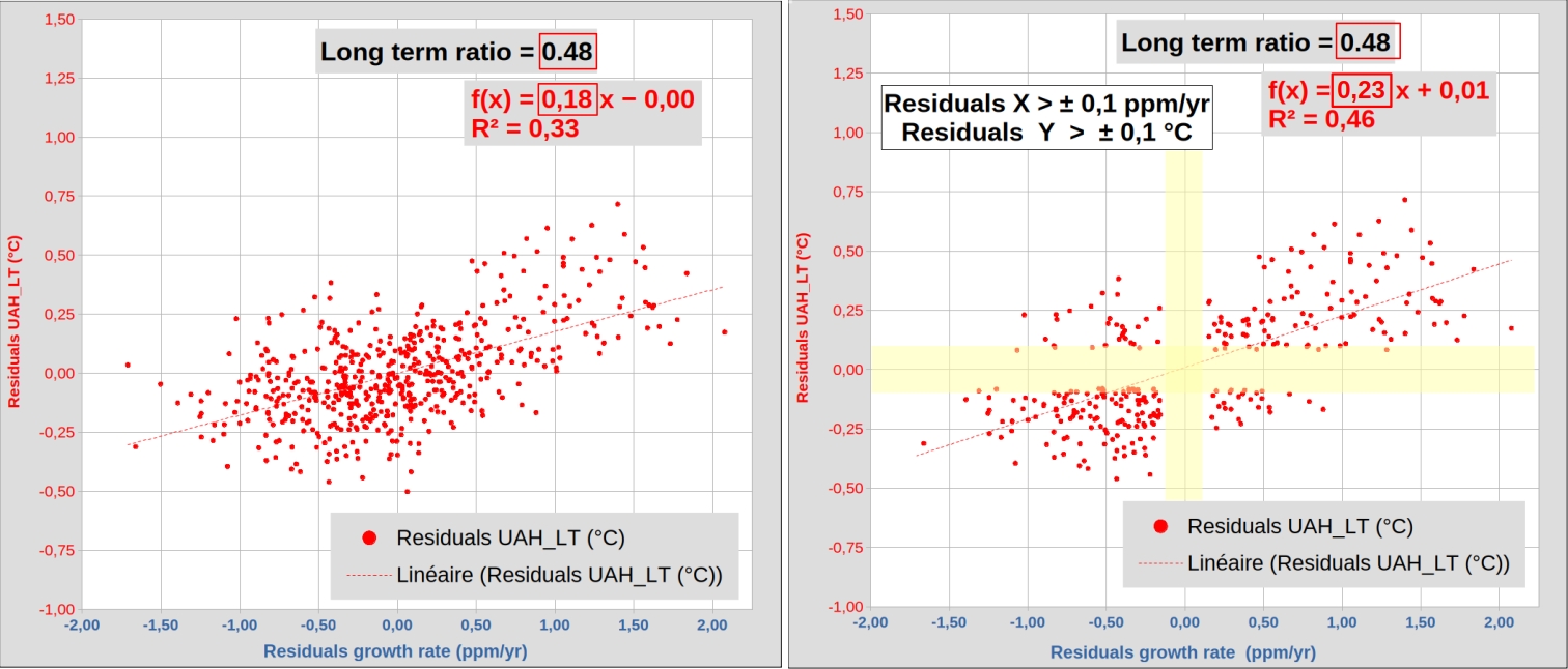
Figure 6c: left, comparison for 100% of residuals; right, comparison for 50% of residuals: their ratio = 0.23, which remains far from the long-term trend ratio = 0.48.

6.3 The IPCC thesis is not compatible with observations

• For annual growth, the IPCC authors (AR6 § 5.21) therefore separate short-term transients (which would be driven by ENSO via flows 3 and 4) from the long-term trend, which would be the result of anthropogenic flow alone (the IPCC multiplies by the trend ratio = 46% designated by Airborne Fraction, see Fig. 3a).

• We recall the result obtained by comparing, after adjustment, anthropogenic flux and atmospheric CO₂ growth: Pearson correlation 0.54 versus 0.73 for UAH_LT_Tropics. For the same detrended series, we have 0.13 versus 0.61 or 0.57 for UAH_LT Tropics. We repeat the procedure illustrated in Fig. 6c, but apply it to the anthropogenic flux: do we find the long-term trend ratio (0.07154/0.0328 = 2.18) by calculating the ratio of residuals (deviations or transients)?

Figure 6d: Two graphs showing anthropogenic flow residuals as a function of annual growth residuals. On the left, 100% of residuals are used; on the right, only 50% of residuals (the largest ones) are retained.

• There is no similarity between the long-term trend ratio (2.18) and the transient ratio (0.04), even when selecting the largest (0.05).
  There is no relationship (R² = 0.02) between annual growth transients and anthropogenic flux transients.
  Correlation does not always imply causation, but the absence of correlation indicates an absence of causality.

• The table below summarizes the analysis of correlations with annual atmospheric CO₂ growth. The analysis does not use the concept of residence time, but only the best observations (544 months between 1980 and 2025).

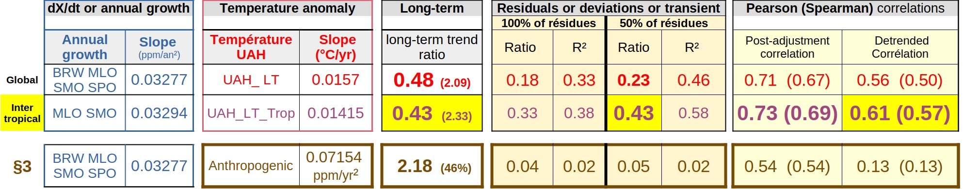
Figure 6e: Summary table of comparisons; the intertropical temperature UAH_LT_Trop shows the best detrended correlation (0.61 or 0.57) and the Δ temperature/Δ annual growth ratios are identical for the long term (0.43) and large transients (0.43).

The main cause of the increase in atmospheric CO₂ does not therefore appear to be anthropogenic emissions; rather, it seems to be linked to variations in temperature in the intertropical zone.
The following paragraph gives additional reasons why “Revisiting the carbon cycle” ultimately favors intertropical ocean surface temperature (SSTi) and flux 1 (Fig. 5d).

 
7. Intertropical ocean degassing is believed to be the main cause of the correlation

7.1 Orders of magnitude

– 75% of the Earth’s surface between 23°26′ S and 23°26′ N is ocean → the temperature of the lower troposphere in the intertropical zone largely reflects the temperature of the ocean SSTi = intertropical Sea Surface Temperature. This is because the heat capacity of the ocean is higher than that of the atmosphere (depending on depth, the ratio is 10 to 1000 here fig.1).
– The carbon stock in the ocean is about 16 times greater than that in vegetation/soils.
– The partial pressure of CO₂ in water at the ocean surface varies greatly depending on its temperature (function of SST^12.5).
The same increase in SST temperature will therefore have a greater effect on flux 1 (warm intertropical zone SST ≈ 25°C to 32°C) than on flux 2 (high latitudes, cold zone SST ≈ 5°C to 15°C). For the same increase of 0.5°C, the reader can verify that 30.5^12.5 – 30^12.5 > 10.5^12.5 – 10^12.5 (the correct calculation in Kelvin yields the same inequality).

7.2 The ¹³C isotope and δ¹³C

• In addition to the above considerations, “Revisiting the carbon cycle” adds modern observations on the ¹³C isotope in the atmosphere: the evolution of δ¹³C cannot be attributed solely to a net anthropogenic carbon input (see §4 here).
An additional net contribution is required: does it come from the Ocean compartment or the Vegetation/Soil compartment?

• With regard to the vegetation/soil compartment, it is likely that plant decomposition (flow 3 in Fig. 5d) increases with temperature. However, plant decomposition is probably lower than carbon absorption by vegetation (flow 4 in Fig. 5d) because the overall greening of the planet suggests that flow 4 > flow 3 → no net input.

• The same increase in temperature has a greater effect on flux 1 (warm zone) than on flux 2 (cold zone) → flux 1 > flux 2 → possible net input. On the other hand, for flux 1 in the intertropical zone, δ¹³C is 1.5‰ lower than that of the atmosphere. A net additional input of carbon from the intertropical ocean to the atmosphere would then balance the δ¹³C budget (‘Revisiting the carbon cycle’ estimates flux 1 in order to close the balance for δ¹³C).

• ‘Revisiting the carbon cycle’ therefore compares annual growth (but observed at MLO) and the intertropical ocean temperature SSTi (but since 1959, therefore excluding satellite observations). In Figure 2, the small anthropogenic contribution is deducted from annual growth: the correlation is then excellent. In Figure 3 (similar to Figure 5b here), the anthropogenic contribution is also deducted. Section 7 and Figures 22, 23, and 24 detail the evolution of δ¹³C from 1980 to 2020.

8. Conclusions

• The model used in “Revisiting the carbon cycle” is based on correlation analysis using the most reliable modern measurements. The weak correlation between anthropogenic flux adjusted via the ‘airborne fraction’ and annual growth calls into question the IPCC’s thesis. On the other hand, the correlation observed between the detrended series suggests that the temperature of the intertropical zone significantly influences annual growth, mainly through natural carbon exchanges (Fig. 6e).

• Regarding natural carbon exchanges in the intertropical zone, other evidence (§7) indicates that the influence of the ocean predominates over that of vegetation and soils. However, the correlation obtained is not perfect: the ocean plays a major role, but other secondary factors also intervene.

• In the natural sciences, it is common practice to quantify correlations by selecting the best available observations and applying signal processing methods. Although the young science of climate is often considered “settled,” why not apply these proven methods to it?

• In the IPCC’s AR6 WG1 report, the term “model” appears 14,192 times, compared to 3,106 occurrences for the term “observation”  (82% vs. 18%). If the IPCC Bureau recognized that observations should guide models, it would select more observers among its editors. Unfortunately, such an aggiornamento would risk undermining the  “scientific consensus” of modelers/editors.

Part 2 of the article presents the model used in Figures 14 and 15 of § 6 of “Revisiting the carbon cycle.”
Part 3 provides illustrations to help better understand the model and answers common objections.

 
References

Revisiting The Carbon Cycle  https://doi.org/10.53234/scc202510/10

[CO₂] according to NOAA  Observatoires de référence  
UAH LT and LT_Tropics  https://www.nsstc.uah.edu/data/msu/v6.1/tlt/uahncdc_lt_6.1.txt
Anthropogenic emissions according to CDIAC
Anthropogenic emissions according to BP statistical review
Anthropogenic emissions according to Carbonmonitor.
SST according to NOAA   https://www.psl.noaa.gov/data/gridded/data.noaa.oisst.v2.highres.html
KNMI Climate explorer  https://climexp.knmi.nl

Le cycle du carbone (Camille Veyres 2024)
The Rational Climate e-Book (section 1.4 page 32) de Patrice Poyet.
Une comparaison absente du rapport du GIEC SCE_01/2025
Addendum.pdf