par J.C. Maurin, Professeur agrégé de physique

2/3  Introduction au modèle MPO

2/3 Introduction to the MPO model (see below)

La revue à comité de lecture Science of Climate Change a publié en 2025 un article intitulé ‘Revisiting the carbon cycle’. Ce travail de 50 pages remet en question de manière globale le cycle du carbone tel qu’il est modélisé par le GIEC. La 1ére partie présente les indices ayant conduit à l’élaboration du modèle proposé dans ‘Revisiting the carbon cycle’, tandis que cette 2éme partie décrit ce modèle.
Selon le GIEC, les échanges naturels de carbone seraient presque équilibrés et relativement constants, tandis que les émissions anthropiques augmentent. Dans cette hypothèse, l’activité humaine serait la seule responsable de la récente hausse du CO₂ atmosphérique. En revanche, le modèle de ‘Revisiting the carbon cycle’ propose des causes Mixtes, à la fois anthropiques et naturelles. Il suggère que les flux de carbone quittant l’atmosphère sont Proportionnels à sa teneur en carbone et que tous les flux auraient augmenté, principalement sous l’effet du dégazage Océanique. Ce modèle, appelé modèle MPO, est brièvement décrit dans cette partie 2, dont la version PDF est disponible ici.

On s’intéresse ici aux évolutions pluriannuelles du CO₂ atmosphérique et non aux évolutions saisonnières. Pour cette raison, adopte un pas temporel de 1 an. On se base exclusivement sur les mesures modernes (MLO à partir de 1959).
Le carbone est présent dans l’atmosphère principalement sous forme de CO₂ : on peut utiliser une unité de masse de CO₂ (1 Gt-CO₂ = 10¹² kg de CO₂), ou bien une proportion relativement à l’atmosphère (1 ppm = partie par million = 0,0001 % → 7,8 Gt-CO₂). Mais de telles unités sont mal adaptées pour les échanges avec l’océan ou la biosphère : on préfère plutôt utiliser ici la masse de carbone (1 Gigatonne de carbone = 1 Gt-C = 1Pg-C = 10¹² kg de carbone → 0,47 ppm → 3,66 Gt-CO₂).

1.  Les ordres de grandeurs

• Afin de se conformer à la modélisation et aux désignations du GIEC, on simplifie le cycle du carbone à des échanges entre 3 compartiments : océan, atmosphère, végétation/sols. Depuis les années 1960, des mesures directes [1] sur plusieurs sites permettent d’avoir une bonne connaissance du stock de carbone dans l’atmosphère = X(t). En revanche, le stock de carbone dans l’océan = Z(t) est seulement estimé, et celui du compartiment Végétation /Sols = Y(t) est mal connu (il est difficile d’estimer la part de carbone du sol qui serait échangeable avec l’atmosphère à l’échelle du siècle).

• Les flux échangés entre les 3 compartiments sont encore plus mal connus (sauf le flux anthropique à ± 5 %) car évalués indirectement via le rapport Stock / Flux sortant. Ce rapport est désigné par : durée de séjour.
  Pour l’atmosphère, les estimations de la durée de séjour sont comprises entre 3 ans et 10 ans [1].
  Par exemple, pour un stock atmosphérique = 870 Gt-C et une durée de séjour = 5,8 ans, alors le flux sortant est estimé à 870 / 5,8 ≈ 150 Gt-C/an (voir tableau ci-dessous : 150 ≈ 79,5 + 71 = flux sortant  = flux 2 + flux 3).
  

 
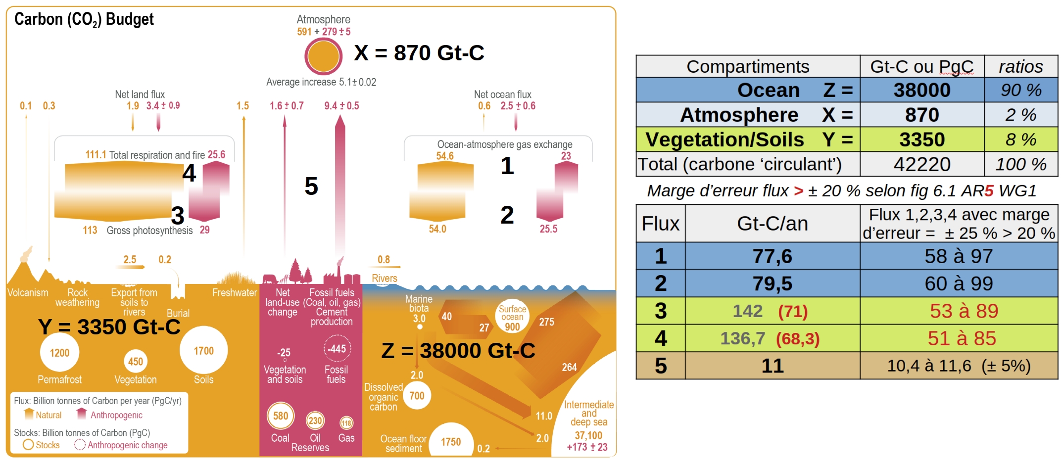
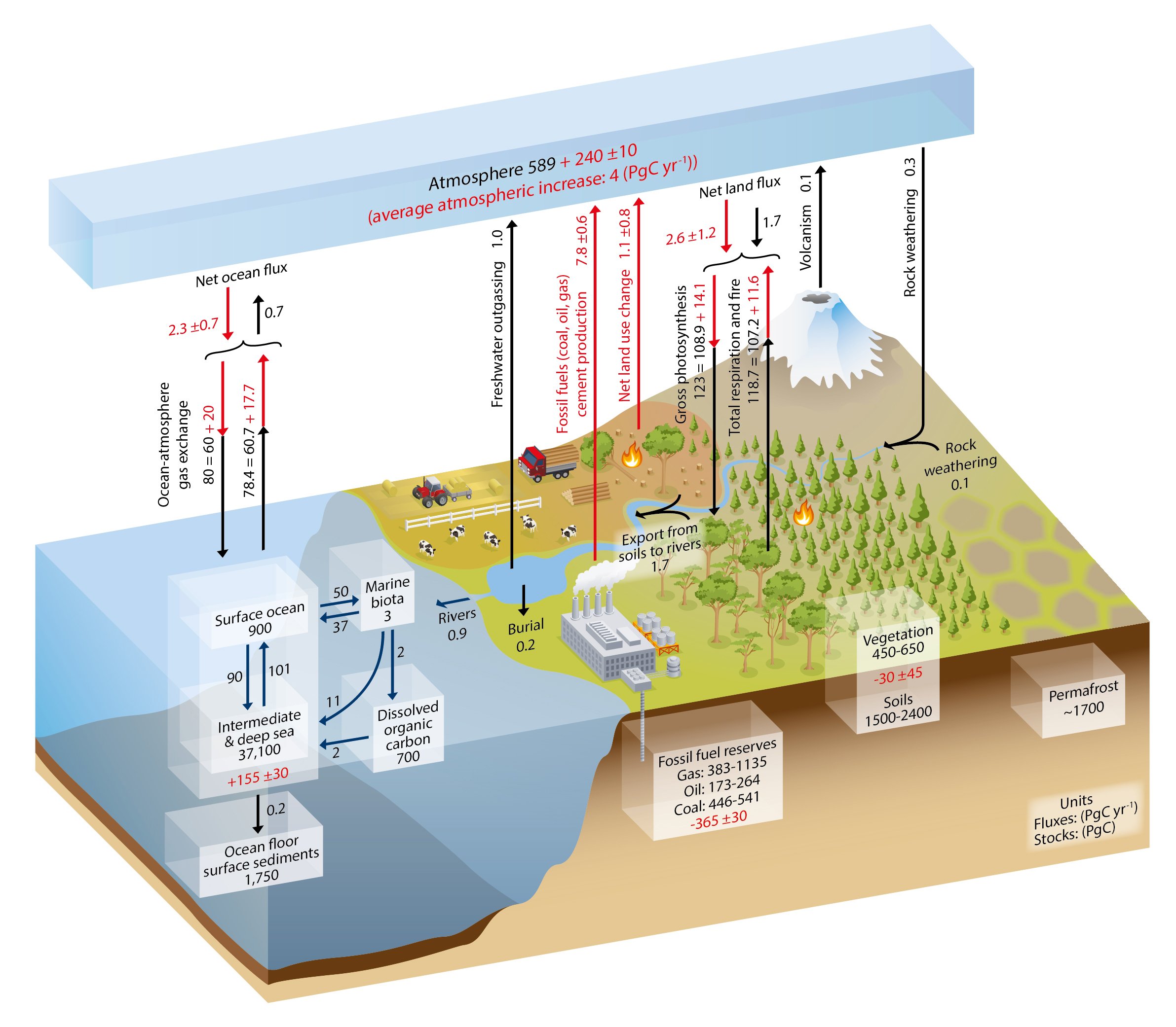
Figure 1 : Estimations GIEC des stocks X Y Z des 3 compartiments (1Gt-C = 1 Pg-C = 10¹² kg de carbone) et des échanges de carbone (Gt-C/an) selon la figure 5.12 publiée dans l’AR6 en 2021. Le tableau à droite résume les estimations du GIEC. Marge d’erreur des flux naturels = ± 25 % > 20 %.

• Par commodité, on a numéroté les 5 flux d’échange de carbone. Dans cette figure 5.12 AR6, le GIEC présente des flux 3 et 4 qui correspondent à la GPP = Gross Primary Production. Cependant, pour la fixation pluriannuelle effective du carbone par la végétation, on doit plutôt utiliser la Net Primary Production → NPP ≈ GPP/2 (voir ici).
  Ce choix du GIEC d’utiliser la GPP plutôt que la NPP tend à surestimer les flux 3 et 4 pour les échanges pluriannuels et donc à sous-estimer le rôle de l’océan (il constitue pourtant 90 % du carbone ‘circulant’). Dans le tableau, les valeurs GPP sont en gris, NPP en rouge.

• En pratique, on peut considérer que 2 compartiments principaux (Z ≈ 90 % et Y ≈ 8 %) échangent du carbone par l’intermédiaire de l’atmosphère (X ≈ 2 %) qui est un simple canal d’échange. Les entrées totales dans l’atmosphère (flux 1+4+5) seraient ≈ 180 Gt-C/an, l’entrée anthropique (flux 5 ≈ 10 Gt-C/an) représenterait ≈ 5 % des entrées totales [2].

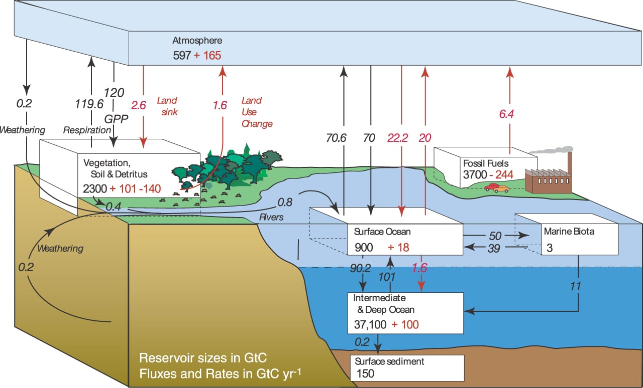
• La figure ci-dessous illustre les tailles relatives des 3 compartiments. On y reporte l’estimation selon le modèle MPO des 3 stocks (désignés par X, Y, Z). Le tableau donne les estimations des 5 flux en 2020 selon le modèle MPO (date proche de la publication de l’AR6 en 2021).
  

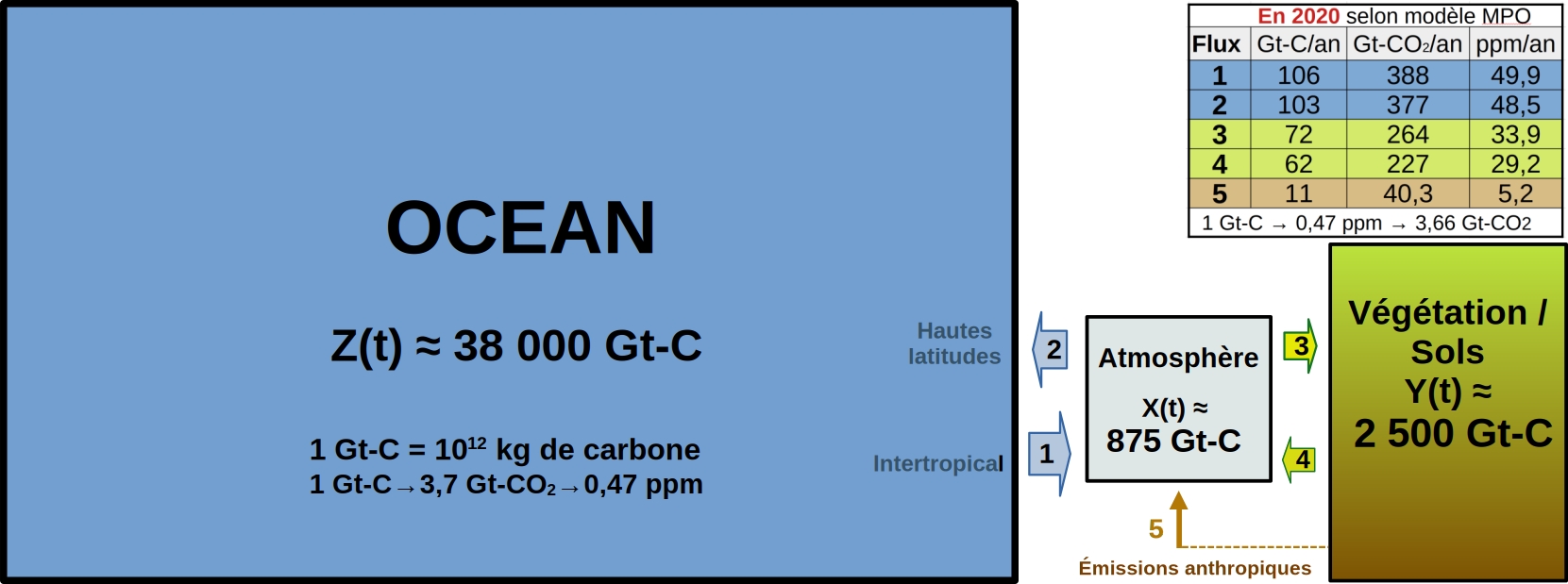
Figure 2 : Estimations (vers 2020 selon le modèle MPO) des stocks X, Y, Z (3 compartiments) et des échanges de carbone (5 flux).

2.  Modèle GIEC et modèle MPO

2.1  Nécessité d’un modèle concurrent à celui du GIEC

• Le modèle GIEC présente de nombreuses incohérences (voir §10 de ‘Revisiting the carbon cycle’).
  – La croissance annuelle du CO₂ atmosphérique (Growth rate) est très mal corrélée avec les émissions anthropiques (ici).
  – Le modèle GIEC ne restitue pas les variations mesurées dans l’atmosphère pour les isotopes ¹³C et ¹⁴C.
  – Le modèle GIEC nécessite que la nature sélectionne (en sortie d’atmosphère) le CO₂ selon son origine : anthropique (flux 5) ou naturelle (flux 1 et 4). En effet, le GIEC prétend que 56 % du CO₂ apporté par le flux 5 quitte l’atmosphère contrairement au CO₂ apporté par les flux 1 et 4 (ici).
  – Le modèle GIEC peine à expliquer le verdissement planétaire (flux 3 quasi constant dans AR2, AR3, AR4, AR5 → fig.4).
  
• Le modèle MPO est guidé par l’observation suivante : la croissance du CO₂ atmosphérique (Growth rate) est bien corrélée avec la température de la zone intertropicale (fig.6e du 1/3 ou fig.2 de ‘Revisiting the carbon cycle’).

2.2  Stocks et flux selon les modèles GIEC ou MPO

• Les stocks X Y Z estimés en 2020 selon le GIEC (fig.1) ou MLO (fig.2) sont similaires, sauf pour Végétation/ Sols. En effet, pour les sols, l’évaluation est très difficile : 2900 Gt-C selon le GIEC contre 2150 Gt-C selon le modèle MPO.

• Le GIEC considère que les flux naturels (1,2,3,4) sont peu variables et équilibrés (voir fig.4 avant 2021) alors que le modèle MPO considère qu’ils sont tous en croissance lors des dernières décennies.

• Le carbone sortant de l’atmosphère se répartirait presque équitablement entre Océan (flux 2) et Végétation/Sols (flux 3).  Selon le GIEC qui utilise la GPP, on a flux 3 > flux 2 ; tandis que l’on a flux 2 > flux 3 selon MPO (ou GIEC en utilisant la NPP).
  
• La comparaison des tableaux des figures 1 et 2 montre que les flux 3,4,5 sont compatibles entre modèles GIEC et MPO, alors que les flux 1 et 2 semblent moins compatibles en 2020 (légende fig. 6.1 AR5 → marge d’erreur supérieure à ±20 %).

• Selon le GIEC, depuis 1959, l’océan serait un puits net de carbone : il absorberait du carbone (flux 2 > flux 1). Ce point est contesté au § 8 de ‘Revisiting the carbon cycle’ : selon MPO, l’océan serait une source nette de carbone (flux 1 > flux 2).
  La baisse du pH océanique moyen serait incompatible avec l’océan = source nette : cette objection sera abordée dans la troisième partie de l’article.
  

3.  Introduction au modèle MPO

• Le présent article est une simple introduction : en 6 pages, il ne peut pas résumer 50 pages de ‘Revisiting the carbon cycle’. Le modèle MPO reprend les 3 compartiments et les 5 flux utilisés par le GIEC dans sa figure 5.12 AR6 WG1. On simplifie ainsi le monde réel pour obtenir une approximation du cycle du carbone à l’échelle de quelques décennies.
  
  
• Le Modèle MPO utilise une hypothèse qui n’est pas en contradiction avec les rapports ARx WG1 du GIEC (voir fig. 4). Le modèle MPO fait l’hypothèse que les flux sortant de l’atmosphère (2 et 3) sont approximativement proportionnels à son contenu en carbone = X(t). La proportion serait de 20 % → chaque année, 1/5 du stock atmosphérique X(t) serait fixé par les compartiments Océan = Z(t) et Végétation/Sols = Y(t). En 5 ans, les flux 2 et 3 extrairaient donc l’équivalent de la totalité du stock atmosphérique → durée de séjour = 5 ans, valeur compatible avec les estimations entre 3 et 10 ans .
    

3.1  Une analogie atmosphère / réservoir

La figure ci-dessous propose une analogie : l’atmosphère se comporterait approximativement comme un réservoir vis-à-vis du CO₂ : le débit de sortie (écoulement par gravité) serait proportionnel à la pression donc à la hauteur X(t) dans le réservoir.

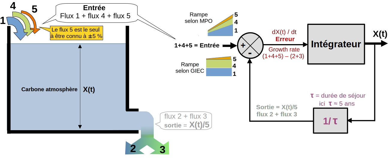
Figure 3a :  à gauche : analogie avec un réservoir → sortie proportionnelle à X(t) → système d’ordre 1 ;  à droite : interprétation selon la science de l’automatique (fig.14 ici)→ dans ce schéma-bloc, le terme ‘Erreur’ désigne la différence entre entrée et sortie du réservoir.

• C’est la différence entre flux d’entrée (1+4+5) et flux de sortie (2+3) qui provoque le changement annuel de X(t) = Growth rate = dX(t)/dt avec dt = 1 an. On note que le seul flux estimé à ± 5 % est le flux 5 (émissions anthropiques ou fossiles).

• En automatique [3], une entrée/commande qui croît quasi linéairement est appelée ‘rampe’. Selon le GIEC, la croissance en entrée (voir les 2 rampes du schéma-bloc fig. 3a) est causée par le seul flux 5. En revanche, selon MPO, elle est causée par les 3 flux : 5, 4, 1, mais principalement par le flux naturel 1 qui entraîne à terme la croissance du flux naturel 4.

• Dans ‘Revisiting the carbon cycle’ le § 4 compare dX(t) /dt = Growth rate avec le flux anthropique 5 → très mauvaise corrélation. La figure 3 compare dX(t)/dt avec la température de la basse atmosphère UAH TLT→ bonne corrélation.
  En supposant que 20 % du carbone (anthropique et naturel) sorte de l’atmosphère chaque année, on peut séparer la part naturelle X_natural et la part anthropique X_fossil. La figure 2 compare alors dX_natural(t) /dt avec la température SSTi  = Sea Surface Temperature intertropical → excellente corrélation. 
  
• ‘Revisiting the carbon cycle’ fait alors l’interprétation suivante : la température SSTi commande le flux 1, qui est le moteur des hausses successives : flux 1→X(t)→flux 2 et flux 3→Y(t)→flux 4 (l’apport de carbone océanique dans l’atmosphère fait croître la végétation).

3.2  Une analogie Growth rate / erreur de traînage

On représente ci-dessous la différence entre les entrées (1+4+5) et les sorties (2+3), qui correspond à la croissance annuelle du CO₂ atmosphérique = Growth rate = dX/dt (dt = 1 an).

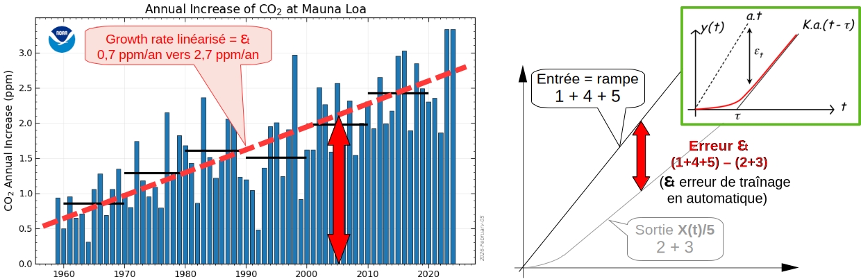
Figure 3b : à gauche : croissance annuelle mesurée à Mauna Loa = Growth rate = ε_t = Erreur selon schéma bloc fig 3a ;  à droite : sortie théorique d’un système d’ordre 1 dont l’entrée est une rampe (l’encadré vert donne les relations liant les pentes d’entrée et de sortie).

• L’observation, depuis le début des mesures à MLO, montre que la croissance annuelle (Growth rate) est très variable, elle est corrélée avec la température, et tend à accélérer : 1960 → 0,7 ppm/an (1,5 Gt-C/an), 2025 → 2,7 ppm/an (5,7 Gt-C/an).
  La tendance (en rouge, fig 3b gauche) montre l’évolution moyenne de Growth rate = dX(t) /dt = Entrée – Sortie.

• La partie droite de la figure suggère, dans le cadre des systèmes asservis et des hypothèses du modèle MPO, une interprétation possible via l’erreur de traînage/vitesse notée ε_t. Entre 1959 et 2025, les entrées croissantes (la cause) ne seraient jamais rattrapées par les sorties qui augmenteraient comme X(t)/5 (la conséquence). L’analogie aide à la compréhension mais reste imparfaite, car le monde réel est moins simple que le schéma-bloc de la fig. 3a.

4. Le modèle MPO

4.1 Une hypothèse qui n’est pas en contradiction avec six rapports du GIEC

L’hypothèse d’une durée de séjour constante = 5 ans (F2 + F3 = X(t)/5) est quasi compatible avec les rapports du GIEC. En effet, le tableau ci-dessous montre que la durée de séjour selon le GIEC varie peu avec la date des rapports ARx et que sa valeur moyenne est comprise entre 3,8 et 5,3 (selon l’utilisation de GPP ou NPP pour F3).

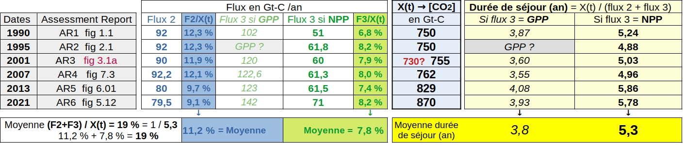
 Figure 4 : Évolution, en fonction de la date, des flux sortant F2 et F3 et de la durée de séjour selon les 6 rapports ARx WG1 du GIEC [1].

Dans le modèle MPO, le carbone sortant de l’atmosphère est supposé = 1/5 ou 20 % du stock X(t) de carbone dans l’atmosphère.
Ce flux sortant se divise en F2 et F3 → 20 % = 11,4 % vers l’océan (F2) + 8,6 % vers Végétation/Sols (F3).
Le GIEC utilise des valeurs proches → 19 % = 11,2 % (F2) + 7,8 % (F3) si on utilise NPP pour F3 (fig.4).
L’hypothèse de départ du modèle MPO est donc quasi compatible avec les 6 rapports scientifiques WG1 du GIEC.
En revanche, les estimations, selon MPO, des flux F1 et F4 entrant dans l’atmosphère s’écartent des estimations du GIEC.

4.2  Les paramètres principaux du modèle MPO

• On reproduit ci-dessous la figure 15 de l’article [2] ‘Revisiting the carbon cycle’ fixant les notations. Son paragraphe 6 présente les équations (équation 12) reliant les différentes grandeurs et déduit leurs évolutions grâce à X(t) mesuré à MLO.

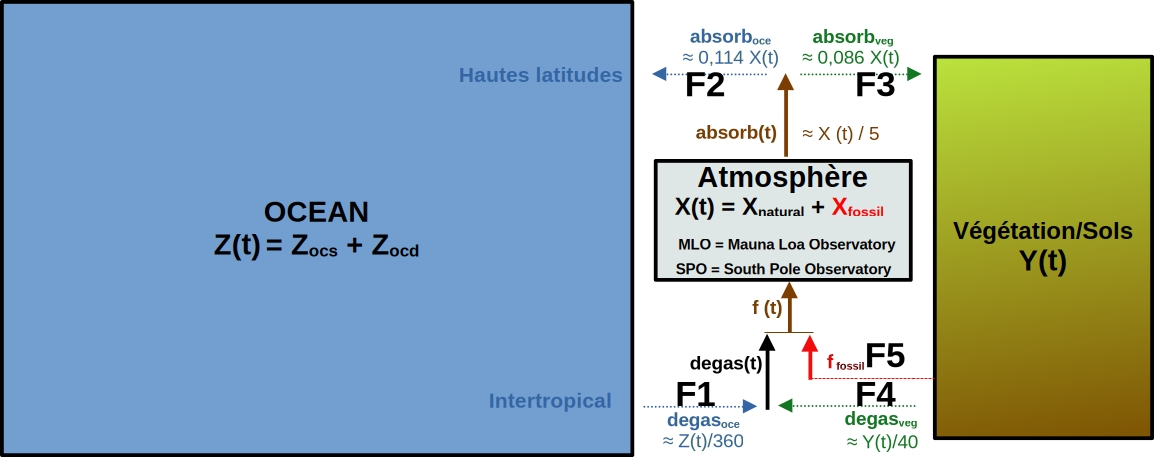
Figure 5 : Le modèle de ‘Revisiting the carbon cycle’ et ses notations, auxquelles on a superposé la précédente numérotation des flux. X(t), Y(t), Z(t) dépendent de la date et représentent les stocks carbone des 3 compartiments : Atmosphère, Végétation/sols, Océan. 

• Les flux 2 et 3 sortant de l’atmosphère correspondent à 11,4 % de X(t) vers l’océan et 8,6 % de X(t) vers Végétation/Sols.

• Le flux 4 provient de la décomposition végétale. On évalue à ≈ 40 ans la durée de séjour moyenne dans Végétation/Sols  → 1/40 du stock Y(t) sort du compartiment chaque année. Si Y(t) croît entre 1959 et 2025, alors F4 augmentera aussi.

• Le flux 1 = Z(t) / 360 provient du dégazage de l’océan intertropical : la durée de séjour dans l’océan serait ≈ 360 ans en 2020. Le § 8 de ‘Revisiting the carbon cycle’ montre que la pression partielle du CO₂ dans l’océan dépend de la température SST et varie selon (SST)^12,5. Il en résulte que la pression partielle dans l’océan intertropical reste supérieure à celle de l’atmosphère entre 1959 et 2025. Le flux 1 augmente, piloté par la température SST à la puissance 12,5.
  Afin de rester conforme à l’évolution mesurée de δ¹³C (elle nécessite un apport net de carbone tel que δ¹³C ≈-13 ‰), l’océan doit fournir un apport net (F1 > F2) qui complète celui des émissions anthropiques.

• Le modèle adopte alors une durée de séjour qui décroît si la température en surface de l’océan intertropical = SSTi augmente. Dans le modèle MPO, le flux 1 est fonction de Z(t) mais aussi de la température SSTi, via une durée de séjour τ_oc  variable (τ_oc ≈ 420 ans vers 1960 et τ_oc ≈ 340 ans vers 2025).
  La méthode d’estimation des 4 flux naturels est détaillé dans Addendum.pdf [4]

4.3  Quelques résultats du modèle MPO

• ‘Revisiting the carbon cycle’ (fig.2) permet une prévision : une baisse de la température océanique SSTi entraînerait la stabilisation ou même la décroissance du niveau de CO₂ dans l’atmosphère.
  La croissance du CO₂ atmosphérique (+ 110,4 ppm entre 1959 et 2025) se répartirait en 87,3 naturels et 23,1 anthropiques.
  Le § 7 montre que cette répartition est parfaitement compatible avec l’évolution mesurée de δ¹³C dans l’atmosphère.
  
• Les résultats du modèle sont présentés au § 6 de ‘Revisiting the carbon cycle’, certains figurent dans le tableau ci-dessous.

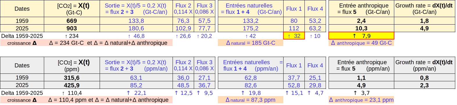
Figure 6 : Les flux en 1959 et en 2025, les valeurs estimées par modélisation figurent en bleu. En haut évolutions en Gt-C, en bas évolutions en ppm. Selon le modèle MPO, entre 1959 et 2025, le dégazage océanique = F1 croît de +32 Gt-C/an contre seulement  +7,9 Gt-C/an pour le flux anthropique.

La troisième partie de l’article illustrera en détail les diverses évolutions (CO₂, δ¹³C, 5 flux, 3 stocks), présentera les bilans globaux pour l’intervalle 1980-2025 et répondra aux objections courantes.

5.  Conclusions

• Les phénomènes naturels sont généralement complexes et très rarement linéaires. De plus, les grandes incertitudes concernant les échanges naturels de carbone rendent toute modélisation incertaine. Dans ce contexte, un modèle ne peut être qu’une simplification de la réalité, une ébauche largement perfectible. 

• Le modèle GIEC adopte une vision fixiste et anthropocentrique (dans l’esprit du modèle astronomique de Ptolémée).
  Son modèle concurrent propose une alternative : une vision dynamique, calibrée sur les mesures fiables modernes.
  Les échanges naturels selon ce modèle sont dans la marge d’erreur (± 25 % sauf pour F1) des estimations du GIEC.

• A l’échelle de quelques décennies, le cycle du carbone peut se résumer à un échange de carbone entre 2 compartiments principaux : Océans→ Z(t) ≈ 90 %  et Végétation/Sols→Y(t) ≈ 8 %  à travers un 3ᵉ compartiment de taille réduite : Atmosphère→X(t) ≈ 2 %. Aux entrées naturelles de carbone dans l’atmosphère, actuellement de l’ordre de 180 (?) Gt-C/an ± 25 % (?), s’ajoute un faible apport anthropique/fossile d’environ 10 Gt-C/an.

• Les mesures à MLO depuis 1959 permettent de montrer que les variations du carbone dans l’atmosphère = dX(t) /dt sont très mal corrélées avec ce faible apport anthropique/fossile. ‘Revisiting the carbon cycle’ (figure 2) montre que dX(t) /dt est au contraire bien corrélé avec la température en zone intertropicale (voir aussi fig.6e dans la partie 1/3).
  La dynamique du CO₂ atmosphérique semble donc surtout régie par des processus naturels : la température de surface de l’océan SSTi (induite par l’insolation), la productivité nette de la végétation et la physico-chimie du carbone dans l’océan.

• ‘Revisiting the carbon cycle’ propose un modèle simplifié pour lequel le carbone sortant annuellement de l’atmosphère serait une proportion (1/5 ou 20%) du stock atmosphérique X(t). On utilise les mesures disponibles récentes (teneur en CO₂, δ¹³C, Δ¹⁴C, température SSTi) pour justifier le modèle et la valeur de ses paramètres. Ce modèle montre alors que :
  a)  L’atmosphère en 2025 est un mélange (natural + fossil) tel que X(2025) = 426 ppm = X_natural+X_fossil = 403 ppm + 23 ppm.
  b)  Entre 1959 et 2025, X(t) croît de +110,4 ppm qui se décomposent en +87,3 ppm naturels et +23,1 ppm anthropiques.
  c)  X_fossil croît lentement (≈ +0,28 ppm/an) alors que X_natural croît 7 fois plus vite (≈ +2 ppm/an depuis l’an 2000).
  d)  Le flux 1 (dégazage océanique) augmente fortement entre 1959 (≈ 80 Gt-C/an) et 2025 (≈ 112 Gt-C/an). En effet, dans l’eau de mer, la pression partielle varie selon la température à la puissance 12,5 et cette température a augmenté.
  e)  Cet apport croissant de carbone océanique dans l’atmosphère (la cause) entraîne ensuite la croissance de la végétation : sa productivité nette (flux 3) augmente entre 1959 (≈ 57 Gt-C/an) et 2025 (≈ 78 Gt-C/an).
  
• Dans  les 10 pages du § 10 de ‘Revisiting the carbon cycle’, il est démontré que de nombreux concepts ou assertions du GIEC/ONU sont illusoires (adjustment time, airborne fraction, IRF de Bern, buffer factor, etc.). Concernant d’autres assertions du GIEC/ONU, le lecteur peut se référer à l’article SCE_03/2025.
  

La partie 1 de l’article expose les raisons qui ont guidé vers le modèle (étude des corrélations et δ¹³C).
La partie 3 de l’article illustre les évolutions 1980-2025 selon le modèle MPO et répond aux objections courantes.

Références

1  CO₂ dans l’atmosphère
Mauna Loa Monthly Averages CO₂
Tom V. Segalstad  http://www.co2web.info/ESEF3VO2.pdf.
Compilation : Sundquist, E.T. 1985: Geological perspectives on carbon dioxide and the carbon cycle.
Échanges de carbone selon les rapports WG1 du GIEC : AR6 Fig 5.12  |  AR5 Fig 6,01  |  AR4 Fig 7.3  |  AR3 Fig 3.1a  |  AR2 p.77 (fig 2.1)  |  AR1 chap.1 p.8  (Fig 1.1)  

2  Articles connexes
Revisiting the carbon cycle (Veyres Maurin Poyet)
What Causes Increasing Greenhouse Gases? (Salby Harde, 2022)
Koutsoyiannis 2024a
Koutsoyiannis 2024b 
Le château de carte du réchauffement anthropique (C. Veyres)
The Rational Climate e-Book: Cooler is Riskier  (P. Poyet).
Examen critique de 7 assertions du GIEC
Une comparaison absente du rapport du GIEC : Émissions anthropiques vs Croissance du CO₂
Réflexions-concernant-la-declaration-sur-lintegrite-de-linformation-en-matiere-de-changement-climatique
Un-consensus-scientifique-qui-ne-veut-plus-rien-dire

3  Éléments d’automatique
Automatique linéaire
Automatique et systèmes asservis
Réponse à une rampe
Performances des systèmes asservis

4  Téléchargement
Addendum, pdf

‘Revisiting the carbon cycle’

2/3 Introduction to the MPO model
 

 
The peer-reviewed scientific journal Science of Climate Change published an article in 2025 entitled ‘Revisiting the carbon cycle’. This 50-page paper comprehensively challenges the carbon cycle as modeled by the IPCC. The first part presents the evidence that led to the development of the model proposed in Revisiting the Carbon Cycle, while the second part describes the model itself. According to the IPCC, natural carbon exchanges are almost balanced and relatively constant, while anthropogenic emissions are increasing. Under this assumption, human activity would be solely responsible for the recent increase in atmospheric CO₂. In contrast, the Revisiting the Carbon Cycle model proposes Mixed causes, both anthropogenic and natural. It suggests that carbon flows leaving the atmosphere are Proportional to its carbon content and that all flows have increased, mainly due to Ocean degassing. This model, called the MPO model, is briefly described in this second part, a PDF version of which is available here.

Here we are interested in multi-year changes in atmospheric CO₂, not seasonal changes. For this reason, we have adopted a time step of one year. We rely exclusively on modern measurements (MLO from 1959 onwards).
Carbon is present in the atmosphere mainly in the form of CO₂: we can use a unit of mass of CO₂ (1 Gt-CO₂ = 10¹² kg of CO₂), or a proportion relative to the atmosphere (1 ppm = parts per million = 0.0001% → 7.8 Gt-CO₂).
However, these units are poorly suited for exchanges with the ocean or the biosphere: here, it is preferable to use carbon mass (1 gigaton of carbon = 1 Gt-C = 1Pg-C = 10¹² kg of carbon → 0.47 ppm → 3.66 Gt-CO₂).

1. Orders of magnitude

• To align with IPCC modeling and terminology, the carbon cycle is simplified to include exchanges between three compartments: ocean, atmosphere, and vegetation/soil. Since the 1960s, direct measurements [1] at several sites have provided a good understanding of the carbon stock in the atmosphere = X(t). However, the carbon stock in the ocean = Z(t) is only estimated, and that of the vegetation/soil compartment = Y(t) is poorly understood (it is difficult to estimate the proportion of soil carbon that could be exchanged with the atmosphere over the course of a century).

• The flows exchanged between the three compartments are even less well understood (except for anthropogenic flow at ± 5%) because they are assessed indirectly via the stock/outflow ratio. This ratio is referred to as the residence time.
For the atmosphere, estimates of the residence time range from 3 to 10 years [1].
For example, if the residence time = 5.8 years and the atmospheric stock = 870 Gt-C, then the outgoing flow is 870 / 5.8 ≈ 150 Gt-C/year (see table below: 150 ≈ 79.5 + 71 = outgoing flows = flow 2 + flow 3).

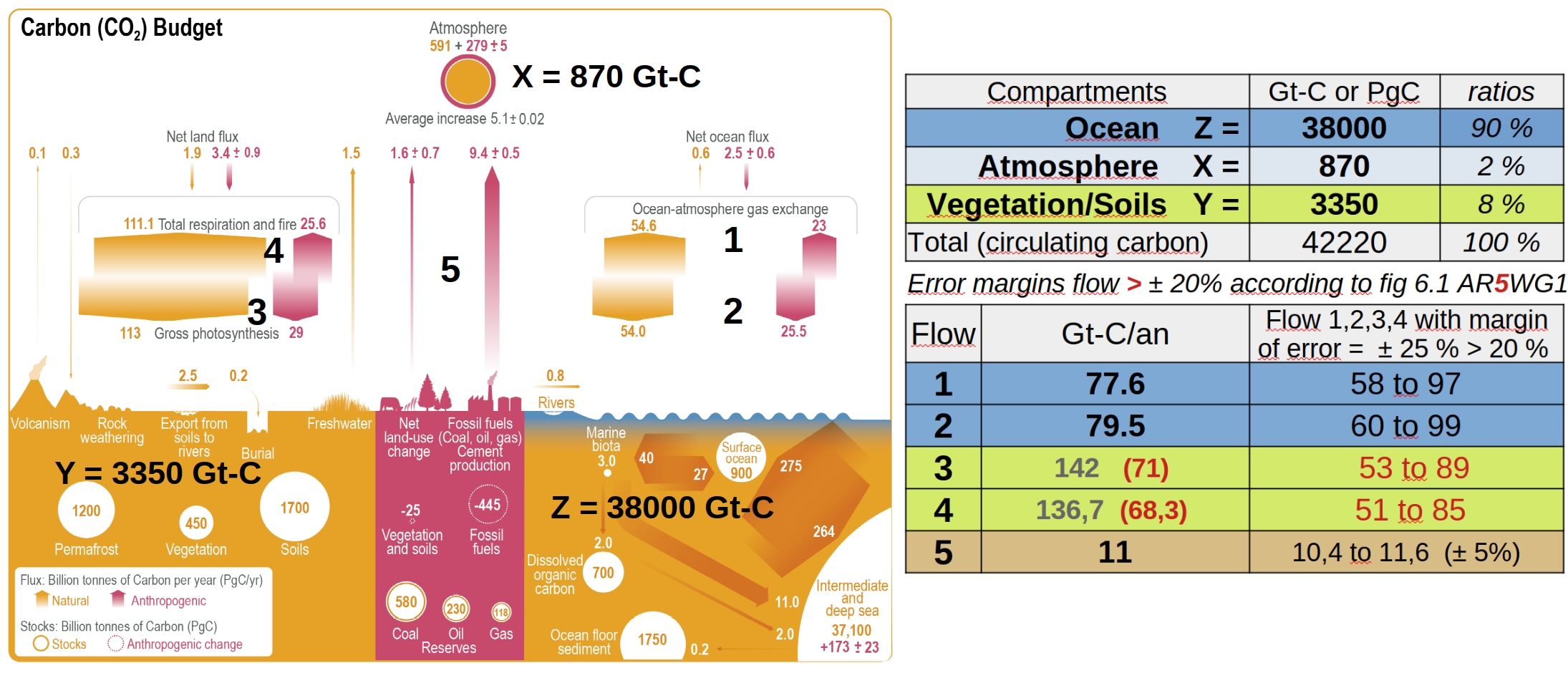
Figure 1: IPCC estimates of X Y Z stocks in the three compartments (1Gt-C = 1 Pg-C = 10¹² kg of carbon) and carbon exchanges (Gt-C/year) according to Figure 5.12 published in AR6 in 2021. The table on the right summarizes the IPCC estimates. Margin of error for natural flows = ± 25% > 20%.

• For convenience, the five carbon exchange flows have been numbered. In Figure 5.12 AR6, the IPCC adopts flows 3 and 4, which correspond to GPP = Gross Primary Production. However, for the effective multi-year carbon fixation by vegetation, Net Primary Production → NPP ≈ GPP/2 should be used instead (see here). The IPCC’s decision to use GPP rather than NPP tends to overestimate flows 3 and 4 for multi-year exchanges and therefore underestimate the role of the ocean (which nevertheless accounts for 90% of ‘circulating’ carbon). In the table, GPP values are shown in gray and NPP values in red.

• In practice, we can consider that two main compartments (Z ≈ 90% and Y ≈ 8%) exchange carbon via the atmosphere (X ≈ 2%), which is simply a channel for exchange. Total inputs into the atmosphere (flows 1+4+5) would be ≈ 180 Gt-C/year, with anthropogenic inputs (flow 5 ≈ 10 Gt-C/year) representing ≈ 5% of total inputs [2].

• The figure below illustrates the relative sizes of the three compartments. It shows the estimates according to the MPO model for the three stocks (designated X, Y, and Z). The table gives the estimates for the five flows in 2020 according to the MPO model (close to the publication date of AR6 in 2021).

 
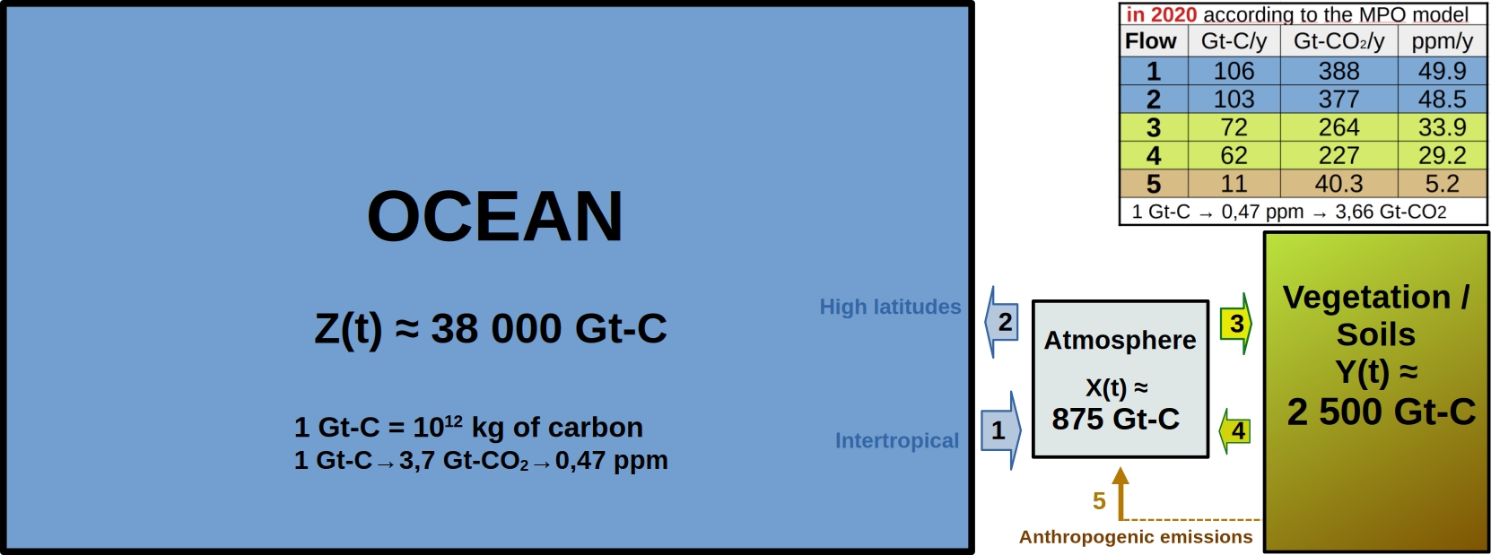
Figure 2: Estimates (around 2020 according to the MPO model) of stocks X, Y, Z (3 compartments) and carbon exchanges (5 flows).

2. IPCC model and MPO model

2.1 Need for a competing model

• The IPCC model has many inconsistencies (see §10 of “Revisiting the carbon cycle”).
– The annual growth rate of atmospheric CO₂ is very poorly correlated with anthropogenic emissions (here).
– The IPCC model does not reproduce the variations measured in the atmosphere for the isotopes ¹³C and ¹⁴C.
– The IPCC model requires nature to select (at the atmosphere’s exit) CO₂ according to its origin: anthropogenic (flow 5) or natural (flows 1 and 4). Indeed, the IPCC claims that 56% of the CO₂ contributed by flow 5 leaves the atmosphere, unlike the CO₂ contributed by flows 1 and 4 (here).
– The IPCC model struggles to explain global greening (quasi-constant flow 3 in AR2, AR3, AR4, AR5 → fig.4).

•  The MPO model is guided by the following observation: the growth rate of atmospheric CO₂ correlates well with the temperature of the intertropical zone (Fig. 6e of 1/3 or Fig. 2 of “Revisiting the carbon cycle”).

2.2 Stocks and flows according to the IPCC or MPO models

• The X, Y, and Z stocks estimated in 2020 according to the IPCC or MLO (Fig. 1&2) are similar, except for Vegetation/Soils. Indeed, for soils, the assessment is difficult: 2,900 Gt-C according to the IPCC versus 2,150 Gt-C according to the MPO model.

• The IPCC considers that natural flows (1, 2, 3, 4) are relatively stable and balanced (see Fig. 4 before 2021), while the MPO model considers that they haveall been growing in recent decades.

• Carbon leaving the atmosphere would be distributed almost equally between the ocean (flow 2) and vegetation/soils (flow 3). This competing model from the IPCC is described here briefly and referred to as the MPO model. According to the IPCC,which uses the GPP, flow 3 > flow 2; whereas according to the MPO (or the IPCC using the NPP), flow 2 > flow 3.

• Comparison of the tables in Figures 1 and 2 shows that flows 3, 4, and 5 are compatible between IPCC and MPO models, while flows 1 and 2 appear to be less compatible in 2020 (legend fig. 6.1 AR5 → margin of error greater than ±20%).

• According to the IPCC, since 1959, the ocean has been a net carbon sink: it absorbs carbon (flow 2 > flow 1). This point is disputed in § 8 of “Revisiting the carbon cycle”: according to MPO, the ocean is a net source of carbon (flow 1 > flow 2).
The decline in average ocean pH would be incompatible with the ocean as a net source: this objection will be addressed in the third part of the article

3. Introduction to the MPO model

• This article is a simple introduction: in 9 pages, it cannot summarize 50 pages of “Revisiting the carbon cycle.”
  The MPO model uses the three compartments and five flows used by the IPCC in Figure 5.12  AR6 WG1.
  This simplifies the real world to obtain an approximation of the carbon cycle over a period of several decades.
  
• To do this, the MPO model uses an assumption that is not inconsistent with the IPCC WG1 ARx reports (see Fig. 4). The MPO model assumes that the flows leaving the atmosphere (2 and 3) are approximately proportional to its carbon content = X(t). The proportion would be 20% → each year, 1/5 of the atmospheric stock X(t) would be fixed by the Ocean = Z(t) and Vegetation/Soils = Y(t) compartments. In 5 years, flows 2 and 3 would therefore extract the equivalent of the entire atmospheric stock → residence time = 5 years, a value compatible with estimates between 3 and 10 years.

3.1 An atmosphere/reservoir analogy

The figure below offers an analogy: the atmosphere would behave approximately like a reservoir with respect to CO₂ : the output flow (gravity flow) would be proportional to the pressure, and therefore to the height X(t) in the reservoir.

 
 
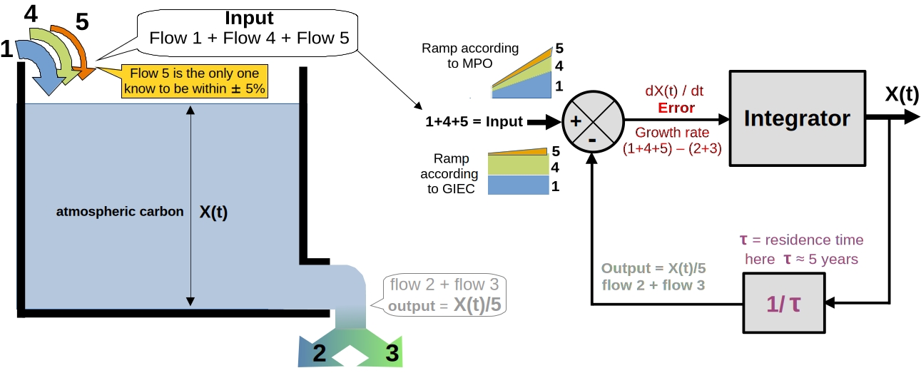
Figure 3a: left: analogy with a reservoir → output proportional to X(t) → first-order system; right: interpretation according to linear control theory (Fig.14 here)→ in this block diagram, the term “Error” refers to the difference between the reservoir’s input and output.

 • It is the difference between input flow (1+4+5) and output flow (2+3) that causes the annual change in X(t) = Growth rate = dX(t)/dt with dt = 1 year. It should be noted that the only flow estimated at ± 5% is flow 5 (anthropogenic or fossil emissions).

• In linear control theory [3], an input/command that grows almost linearly is called a “ramp”. According to the IPCC, the growth in input (see the two ramps in the block diagram in Fig. 3a) is caused solely by flow 5. However, according to MPO, it is caused by the three flows : 5, 4, 1, but mainly by natural flow 1, which ultimately leads to the growth of natural flow 4.

• In “Revisiting the carbon cycle”, § 4 compares dX(t)/dt = Growth rate with anthropogenic flow 5 → very poor correlation. Figure 3 compares dX(t)/dt with lower atmospheric temperature UAH TLT→ good correlation.
Assuming that 20% of carbon (anthropogenic and natural) leaves the atmosphere each year, we can separate the natural portion X_natural and the anthropogenic portion X_fossil. Figure 2 compares dX_natural(t)/dt with the intertropical sea surface temperature SSTi → excellent correlation.
 
• “Revisiting the carbon cycle” then makes the following interpretation: the SSTi temperature controls flow 1, which is the driver of successive increases: flow 1→X(t)→flow 2 and flow 3→Y(t)→flow 4 (the contribution of ocean carbon to the atmosphere causes vegetation to grow).

3.2 An analogy between growth rate and tracking error

The difference between input (1+4+5) and output (2+3) is shown below, which corresponds to the annual growth of atmospheric CO₂ = growth rate = dX/dt (dt = 1 year).

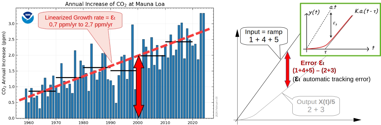
Figure 3b: left: annual growth measured at Mauna Loa = Growth rate = εt = Error according to block diagram fig 3a; right: theoretical output for a first-order system whose input is a ramp (the green box shows the relationships between the input and output slopes).

• Observations since measurements began at MLO show that the annual growth rate is highly variable, correlates with temperature, and tends to accelerate: 1960 → 0.7 ppm/year (1.5 Gt-C/year), 2015 → 2.7 ppm/year (5.7 Gt-C/year).
The trend (in red, Fig. 3b left) shows the average change in growth rate = dX(t) /dt = Input – Output.

• The right-hand side of the figure suggests, within the framework of linear automation and the assumptions of the MPO model, a possible interpretation via the tracking error noted ε_t. Between 1959 and 2025, the increasing inputs (the cause) would never be caught up by the outputs, which would increase as X(t)/5 (the consequence). The analogy aids understanding but remains imperfect because the real world is less simple than the block diagram in Fig. 3a.

 
4. The MPO model

4.1. A hypothesis that is not inconsistent with six IPCC reports

The hypothesis of a constant residence time = 5 years (F2 + F3 = X(t)/5) is fairly consistent with the IPCC reports. Indeed, the table below shows that the IPCC residence time varies little with the date of the ARx reports and that its average value is between 3.8 and 5.3 (depending on whether GPP or NPP is used for F3).

 
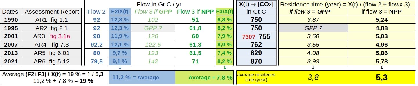
Figure 4: Evolution, over time, of outflows F2 and F3 and residence time according to IPCC WG1 reports [1].

In the MPO model, carbon leaving the atmosphere is assumed to be equal to 1/5 or 20% of the stock X(t) of carbon in the atmosphere. This outflow is divided into F2 and F3 → 20% = 11.4% to the ocean (F2) + 8.6% to vegetation/soils (F3).
The IPCC (Fig. 4) uses similar values → 19% = 11.2% (F2) + 7.8% (F3) if NPP is used for F3.
The initial assumption of the MPO model is therefore fairly consistent with the six WG1 scientific reports of the IPCC.
However, the F1 and F4 flows entering the atmosphere (according to MPO) differ from IPCC estimates.   

4.2 The main parameters of the MPO model

• Figure 15 from article [2] “Revisiting the carbon cycle” is reproduced below, setting out the notations. Paragraph 6 presents the equations (equation 12) linking these different quantities and deduces their changes using X(t) measured at MLO.

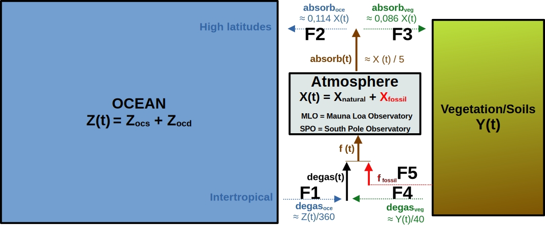
Figure 5: The “Revisiting the carbon cycle” model and its notations, superimposed on the previous flow numbering.X(t), Y(t), Z(t) depend on the date and represent the carbon stocks of the three compartments: Atmosphere, Vegetation/Soils, and Ocean.

• Flows 2 and 3 leaving the atmosphere correspond to 11.4% of X(t) to the ocean and 8.6% of X(t) to Vegetation/Soils.

• Flow 4 comes from plant decomposition. The average residence time in Vegetation/Soils is estimated at 40 years → 1/40 of stock Y(t) leaves the compartment each year. If Y(t) increases between 1959 and 2025, then F4 will also increase.

• Flow 1 = Z(t) / 360 comes from ocean degassing: the residence time in the ocean would be ≈ 360 years in 2020. Section 8 of “Revisiting the carbon cycle” shows that the partial pressure of CO₂ in the ocean depends on the SST temperature and varies according to (SST)^12.5. As a result, the partial pressure in the intertropical ocean remains higher than that of the atmosphere between 1959 and 2025. Flow 1 therefore increases, driven by SST temperature to the power of 12.5. In order to satisfy the measured evolution of δ¹³C (which requires a net carbon input such that δ¹³C ≈ -13‰), the ocean must provide a net input (F1 > F2) that supplements that from anthropogenic emissions.

• The model then adopts a residence time that decreases if the intertropical ocean surface temperature = SSTi increases. In the MPO model, flow 1 is a function of Z(t) but also of the SSTi temperature, via a variable residence time τ_oc (τ_oc  ≈ 420 years around 1960 and τ_oc  ≈ 340 years around 2025).
The method for estimating the four natural flows is detailed in Addendum.pdf [4].

4.3 Some results from the MPO model

• ‘Revisiting the carbon cycle’ (fig.2) allows for a prediction: a deacrease in ocean temperature (SSTi) would lead to stabilization or even a decrease in the level of CO₂ in the atmosphere. The increase in atmospheric CO₂ (+110.4 ppm between 1959 and 2025) would be divided into 87.3 natural and 23.1 anthropogenic. Section 7 shows that this distribution is perfectly compatible with the measured evolution of δ¹³C in the atmosphere.

• The model results are presented in section 6 of “Revisiting the carbon cycle,” some of which are shown in the table below.

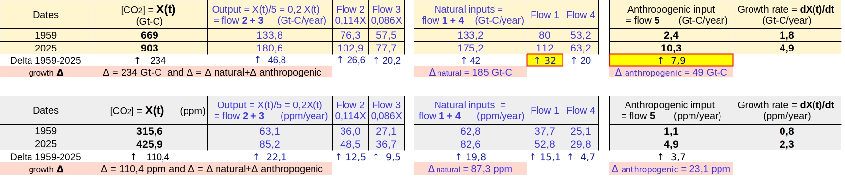
Figure 6: Flows in 1959 and 2025, with values calculated by modeling shown in blue. Top: changes in Gt-C; bottom: changes in ppm. According to the MPO model, between 1959 and 2025, F1 = ocean degassing will increase by +32 Gt-C/year, compared with only +7.9 Gt-C/year for anthropogenic flows.

• The third part of the article will illustrate in detail the various developments (CO₂, δ¹³C, 5 flows, 3 stocks), present the overall balances for the period 1980-2025, and respond to common objections.

5. Conclusions

•  Natural phenomena are generally complex and very rarely linear. Furthermore, the considerable uncertainties surrounding natural carbon exchanges make any modeling uncertain. In this context, a model can only be a simplification of reality, a draft that could be greatly improved.

• The IPCC model adopts a fixed and anthropocentric view (in the spirit of Ptolemy’s astronomical model).
Its competing model offers an alternative: a dynamic view, based on reliable modern measurements. Natural exchanges according to this model are within the margin of error (± 25% except for F1) of IPCC estimates.

 • The carbon cycle over a period of several decades can be summarized as an exchange of carbon between two main compartments: Oceans→ Z(t) ≈ 90% and Vegetation/Soils→Y(t) ≈ 8% through a third, smaller compartment: Atmosphere→X(t) ≈ 2%. In addition to natural carbon inputs into the atmosphere, currently around 180 (?) Gt-C/year ± 25% (?), there is a small anthropogenic/fossil input of around 10 Gt-C/year.

• Measurements at MLO since 1959 show that variations in atmospheric carbon = dX(t) /dt are very poorly correlated with this low anthropogenic/fossil input. “Revisiting the carbon cycle’ (Figure 2) shows that dX(t)/dt is, in fact, strongly correlated with temperature in the intertropical zone (see also Fig. 6e in Part 1/3).
The dynamics of atmospheric CO₂ therefore seem to be governed mainly by natural processes : the surface temperature of the ocean SSTi (induced by insolation), the net productivity of vegetation, and the physical chemistry of carbon in the ocean.

• ‘Revisiting the carbon cycle’ proposes a simplified model in which the carbon leaving the atmosphere each year would be a proportion (1/5 or 20%) of the atmospheric stock X(t). Recent available measurements (CO₂ content, δ13C, Δ14C, SSTi temperature) are used to justify the model and the value of its parameters. This model shows that:
a) The atmosphere in 2025 is a mixture (natural + fossil) such that X(2025) = 426 ppm = Xnatural+Xfossil = 403 ppm + 23 ppm.
b) From 1959 to 2025, X(t) increases by +110.4 ppm, which breaks down into +87.3 ppm natural and +23.1 ppm anthropogenic.
c) Xfossil increases slowly (≈ +0.28 ppm/year) while Xnatural increases seven times faster (≈ +2 ppm/year since 2000).
d) Flow 1 (ocean degassing) increases sharply between 1959 (≈ 80 Gt-C/year) and 2025 (≈ 112 Gt-C/year).  In fact, in seawater, the partial pressure varies with temperature to the power of 12.5, and that temperature has risen.
e) This increasing supply of ocean carbon into the atmosphere (the cause) then leads to the growth of vegetation : its net productivity (flow 3) increases between 1959 (≈ 57 Gt-C/year) and 2025 (≈ 78 Gt-C/year).

• In the article “Revisiting the carbon cycle” (see the 10 pages of § 10), it has been demonstrated that many of the concepts or assertions made by the IPCC/UN are illusory (adjustment time, airborne fraction, Bern IRF, buffer factor, etc.). For further information on other IPCC/UN assertions, readers may refer to article SCE_03/2025.

Part 1 of the article explains the reasons behind the model (study of correlations and δ13C).
Part 3 of the article illustrates the changes between 1980 and 2025 according to the MPO model and responds to common objections.

 
References

1  CO₂ in the atmosphere
Mauna Loa Monthly Averages CO₂
Tom V. Segalstad  http://www.co2web.info/ESEF3VO2.pdf.
Compilation : Sundquist, E.T. 1985: Geological perspectives on carbon dioxide and the carbon cycle.
Carbon exchanges according to IPCC WG1 reports : AR6 Fig 5.12  |  AR5 Fig 6,01  |  AR4 Fig 7.3  |  AR3 Fig 3.1a  |  AR2 p.77 (fig 2.1)  |  AR1 chap.1 p.8  (Fig 1.1)  

2  Related articles
Revisiting the carbon cycle (Veyres Maurin Poyet)
What Causes Increasing Greenhouse Gases? (Salby Harde, 2022)
Koutsoyiannis 2024a
Koutsoyiannis 2024b 
Le château de carte du réchauffement anthropique (C. Veyres)
The Rational Climate e-Book: Cooler is Riskier  (P. Poyet).
Examen critique de 7 assertions du GIEC
Une comparaison absente du rapport du GIEC : Émissions anthropiques vs Croissance du CO₂
Réflexions-concernant-la-declaration-sur-lintegrite-de-linformation-en-matiere-de-changement-climatique
Un-consensus-scientifique-qui-ne-veut-plus-rien-dire

3  Control or automation elements
Linear time invariant system
Linear control theory
Ramp response
Control systems/system Metrics

4  Download
Addendum.pdf